Costly Communication

1. COMMUNICATION AND ORGANIZATION

In 1962 Marshall McLuhan predicted the "Global Village” a world in which communication technology has rendered geographical distance meaningless (McLuhan 1962). With the recent advent of the "World Wide Web” his prediction has become more or less a reality. On the Web, information access is instantaneous, independent of the information's location and type. It is already possible to transmit low resolution video over the Web and the speed and capacity of transmission continue to improve at a rapid pace. 1

Past improvements in communication technology, such as the telegraph, have contributed to significant changes in the organization of economic activity (Chandler 1977). The current and future improvements are likely to have equally profound effects. Unfortunately, the ability to analyze the past changes and predict the future ones is constrained by the limited theoretical understanding of how the cost of communication affects organizational design. The current paper proposes a novel way of modeling communication based on communication protocols that addresses several shortcomings of existing models.

The paper is structured as follows: Section 2 discusses the relation of the proposed approach to the existing literature; Section 3 introduces the basic modeling strategy of examining communication protocols which are represented as binary trees; Section 4 presents assumptions about the costs and benefits of communication; Section 5 analyzes communication protocols given the assumptions; Section 6 examines some anecdotal evidence on communication in organizations in light of the results of the analysis; and Section 7 summarizes the contributions and possible next steps.

1 Advances in transmission technology, such as digital telephone lines and cable modems, are bringing fast and high capacity connections to homes as well.

2. THE NEED FOR A NEW APPROACH TO MODELING COMMUNICATION

2.1 Background

The existing theory of communication in organizations is highly fractured. Many different perspectives ranging from computer science (e.g. Malone and Smith 1988) to sociology (e.g. Yates and Orlikowski 1992) have been brought lo bear on the topic. In economics, two broad streams of theory have been dominant: the message-space literature and the team-theory literature. Both of these streams, as well as some other existing economic models, have important shortcomings, which are summarized below. An excellent overview can be found in Van Zandt (1997).

2.2 The Message-Space Literature

The message-space models are built around iterative communication protocols on Euclidean message spaces (see Hurwicz (1986) for an extensive exposition). The cost of communication is measured as the dimensionality of the minimal message space. This approach results in two shortcomings. First, the dimensionality is difficult to relate to the properties of actual communication channels and hence to changes in the available technology. Second, in order to prevent "information packing," i.e. the approximate encoding of several real numbers into a single one, smoothness assumptions must be imposed. These assumptions are essentially arbitrary and result in solutions that are excessively complex when compared to information packing alternatives. 2

2.3 The Team Theory Literature

The team theory models consider finite exchanges of information in which the actors employ statistical decision theory (see Marschak and Radner 1972). The shortcoming here is that only fixed communication protocols are considered for which the actors optimize their decision rules. With costly communication, the protocol itself is an important choice variable and holding it fixed imposes an arbitrary constraint.3

2.4 Other Economic Models

A variety of other models have been analyzed, which all tend to make ad-hoc assumptions about the cost of communication. There are few exceptions, such as Green and Laffont (1986) and Segal (1996), which are grounded in information theory as pioneered by Shannon (1948). ITiose papers follow the direction taken by computer science beginning with the work of Yao (1979) by focusing on the asymptotic properties of communication protocols. Given the speed of communication inside a computer system, it is appropriate to examine whtf-her the asymptotic complexity of a particular protocol is polynomial or exponential. For communication by human agents, however, the small number properties of communication are more relevant, since each message involves significant effort.

2 See Green and Laffont (1987) for an example of this problem. Given the smoothness assumption, the cost-constrained solution requires the agents to optimize over a space of functions. An information packing alternative is not only straightforward, but also achieves the unconstrained optimum arbitrarily closely.
3 Team theory is really a study of optimal decision making and not a study of optimal communication.

2.5 An Optimal Finite Protocol Approach

The existing literature thus has a gap: there are no models that study finite communication protocols and are grounded in information theory. The current paper therefore proposes a new approach, which determines the optimal finite protocol for a given situation with costly communication. The properties of the optimal protocols are shown to provide important insights into the nature of communication in organizations.

The approach differs from the message-space literature by focusing on discrete message spaces and finite protocols. It differs from the team theory literature by determining optimal protocols rather than keeping the protocol fixed. Finally, it differs from the communication complexity approach by considering small number properties. The next section sets out the modeling approach and defines the basic elements.

3. MODELING APPROACH AND ELEMENTS

3.1 Modeling Strategy Overview

A communication protocol can be represented as a tree, much like an extensive form game. Each tree induces a partition on a state space (exact definitions are given in the following sections). A tree with more branches induces a finer partition which corresponds to having better information available. The gross benefits from better information have to be balanced with the higher cost of designing and using a more complex protocol. The paper addresses two challenges:

  • First, assumptions have to be made for assigning both benefits and costs to different communication protocols. The assumptions have to reflect the particularities of communication in organizations as opposed to computer or telephone systems. The assumptions also have to be flexible enough to accommodate various situations, while imposing sufficient structure to yield results. A possible set of assumptions is presented in Section 4.
  • Second, a method is required for finding the optimal communication protocol. The space of all possible binary trees is both large and discrete, making the search for a tree that maximizes the net benefit of communication difficult. The solution proposed here is a greedy algorithm, which is discussed in Section 5.

The relevant concepts will now be introduced. For simplicity, the case of one-directional communication will be considered.4

3.2 Model Structure for One-Directional Communication

There are two risk-neutral team members, X and Y. The order of events is as follows:

  1. X and Y design a communication protocol y (as defined below), incurring a cost of design of D(ψ).
  2. X observes some information, which is the realization of a state s e S, where S is a finite set of states. A uniform probability distribution over the states in S will be assumed throughout.
  3. X communicates the information to Y using the protocol yf incurring a cost of C(ψ, s).
  4. Y takes an action a from a є A, where A is a finite set of actions.
  5. A benefit G(a, s) is realized, which depends on both the action and the realized state. The benefit function will be assumed to be bounded for all actions and all states.
  6. Steps 2 through 5 are repeated n times.

The objective is to design a communication protocol that maximizes the profit, i.e. the benefit of communication net of the cost of designing and using the communication protocol.

4 The possibility of extending this approach to bi-directional communication is discussed In Section 7.

3.3 Example

Suppose that the set of possible states is S = {1,2,3,4,5,6,7,8). The set S is assumed to be common knowledge between X and Y. The purpose of a protocol is for X to be able to communicate to Y information about which state s e S was realized. Following the established approach in information theory, communication protocols will be modeled as binary trees. Figure 10 shows one possible protocol, where the notation U{-} stands for the uniform distribution over a set.

The nodes of the tree are labeled with the information available to Y. Prior to any communication (the root of the tree), Y only knows that there is a uniform distribution over the set of possible states. If X sends a 0, this indicates that the realized state belongs to the subset {1,2,3} whereas a 1 indicates that it belongs to the subset {4,5,6,7,8). Upon receiving either message, Y updates the probability distribution accordingly as indicated at the child nodes.

The internal nodes of the tree can be thought of as X answering Yes-No questions about the observed realization. Each answer results in the "bisection" of a subset E of the set of possible states S. For instance, consider the node with Y: U{l, 2,3} in the left branch of the tree in Figure 10. At this point the next Yes-No question could be phrased as nIs the realized state s in the subset {2, 3} ?" The answer bisects the subset {1,2,3} into the two smaller subsets {1} and {2,3}.

3.4 Definitions

Several concepts used throughout the analysis will now be defined formally, starting with the definition of a bisection.

Definition: E1 and E2 form a bisection of E, if and only if E, ∩ E2 = Ø and Ej U E2 = E.

Using the definition of bisection, it is easy to define a communication protocol as follows:
Definition: A communication protocol over the set S is a binary tree y, such that

  1. The root node of ψ is S.
  2. Each non-terminal (internal) node has exactly two child nodes.
  3. The child nodes form a bisection of the parent node.

From this definition, it follows immediately5 that the terminal nodes of a communication protocol ψ form a partition of S, which will be denoted as ψ (S). The subset within the partition that contains state s will be written as ψ1(S), i.e. s € ψ2(S). In Figure 10, the partition is ψ (S) = {{1}, {2, 3}, {4,5,6,7,8}} and ψ3(S) = {4, 5,6,7,8}.

When the protocol is used, the realized state s determines the path through the tree. It will be assumed throughout, unless noted otherwise6 that all answers to the protocol questions are given truthfully. Each path results in a unique sequence of 0's and 1’s.

Definition: A path m (ψ, s) is the sequence of bisections that occurs as the protocol tree ψ is traversed for the realization s.

The notation m1(ψ, s) will be used to refer to the i-th bisection along the path. For the protocol in Figure 10, m2(ψ, 2) is the bisection of E = {1,2,3} into E1 = {1) and E2 = {2,3}. The notation I m(ψ, s) I will be used to refer to the length of the path, so that for the protocol in Figure 10 I m(ψ, 2) I =2.

5 A simple inductive argument establishes this property.
6 See Sections 6.2 and 7 for discussions of this assumption.

4. THE COSTS AND BENEFITS OF COMMUNICATION

4.1 The Need for Assumptions Specific to Communication in Organizations

Information theory was originally motivated by the study of the physical transmission of information, specifically in the then emerging telephone and telegraph networks (Shannon 1948). More recently, it has been applied extensively to the study of communication in computer systems (Yao 1979). This technical orientation has shaped the assumptions made about the costs and benefits associated with protocols. Since the transmission of individual bits is extremely fast and low cost, the focus has been on studying the asymptotic properties of protocols. Furthermore, the technical orientation aiso resulted in taking the need to communicate a certain amount of information as given and focusing on the least cost way of accomplishing the transmission. Hence, the benefits of communication were not modeled explicitly.

In this paper, the information theory approach of modeling communication protocols as binary trees will be applied to organizations. The transmission of information in organizations involves not just tele­communications equipment but also human decision makers, who must send and receive the information. A single bisection in the binary protocol tree will therefore not be interpreted literally as a single bit. Instead, a bisection will be interpreted as a message segment that requires significant human effort. This assumption in turn requires including the benefits of communication in the analysis. In the organizational context, whether or not a message segment is sent depends on both its cost and its benefits.

The purpose of this section is to propose a set of assumptions for associating costs and benefits with different protocols. The assumptions are a first cut at addressing some of the specific aspects of communication in organizations. Further work on identifying reasonable assumptions will be required.

4.2 The Cost of Protocol Design

Before a communication protocol can be used, it must first be designed. In the tree representation, the cost of designing a protocol is the cost of coordinating the questions at each non-terminal node. Both X and Y have to agree on what a message segment7 means at any point in the protocol. For communication in organizations, this effort should not be interpreted literally as the design of questions. Nevertheless, even casual observation suggests that organizations expend considerable effort on designing many aspects of communication, such as the timing (e.g. the frequency of a report), the recipients (e.g. the distribution list of a report), and the structure of content (e.g. the format for a report).

Clearly, a more complex protocol should have a higher cost of design. The marginal cost of design will be assumed to be constant per bisection, The cost of protocol design is thus given by

D(ψ) = d . N(ψ)

where N(ψ) is the number of non-terminal nodes for the tree ψ. For instance, the protocol in Figure 10 has three internal nodes so that N(ψ) = 3. One might object that coordinating the bisection of a large set should require a greater effort than for a small set. This issue is addressed below together with assumptions for the cost of using the protocol.

7 Represented by a 0 or a 1 in the protocol.

4.3 The Cost of Coding

When the protocol is used, the sender of a message segment has to answer a question and the receiver has to interpret the answer. In the organizational setting, the sender's effort can broadly be described as the encoding of information and the receiver's effort as the decoding. Assuming the existence of a cost for coding (encoding and decoding) is an important departure from the traditional information theory approach, which considers only the cost of transmission. This assumption also differs from the standard use of state spaces for representing uncertainty in economics, where individuals know effortlessly which state has been realized.8 For the broader organizational interpretation of protocols chosen in this paper, however, coding effort can not be ignored: turning an observation into a message (sender) or a message into information (receiver) requires significant effort.

The cost for the bisection of a set E will be assumed to depend on the probability distribution between the two resulting subsets Ex and E2. Let p be the probability that the answer identifies E], then 1 - p is the probability that the answer identifies E2. It will be assumed that the cost for coding (i.e. encoding and decoding combined) is determined by the binary entropy 9

h(p) = - p • Iog2 p - (1-p) • log2 (1-p)

so that the cost is highest when both subsets are equally likely and decreases as one subset becomes more likely than the other. The cost of coding is then assumed to be linear in the sum over the bisections along a path


where the subscript C indicates the cost of coding. For instance, for the protocol in Figure 10, CC(ψ, 2) = cc • [h(3/8) + h(l/3)].

Making the cost of coding depend on the question, whereas the cost of design was assumed to be constant per question, can be justified as follows.

Designing a question requires creating both subsets E1 and E2. Coding, however, requires only examining the smaller of the two subsets (assume without loss of generality, that E1 is smaller). This suggests that for a given E, the cost of design is constant since |E1| + |E2| = |E|, whereas the cost of coding varies with |E1|. The remaining question is whether the design and coding cost should depend on absolute size, i.e. |E| and |E1|, or on relative size, i.e. |E| / |E| =1 and |E1| / |E| = p (due to the assumed uniform distribution over the elements). Relative size was assumed for two reasons. First, relative size will be seen to result in a simple and intuitive expression for the total cost of coding for a protocol. Second, relative size makes the model immune to "scaling" the state space, e.g. by splitting every state into 100 smaller states, which should not affect the results of the analysis.

8 See for instance Kreps (1990).
9 The choice of the binary entropy is motivated by information theory and turns out to result in a compact expression for the total cost of coding. Examining alternative assumptions will be an important area for further research.

4.4 The Cost of Transmission

Finally, sending the answer to a question requires the transmission of a message segment. Separating the cost of coding from the cost of transmission will be seen to be important for the interpretation of results. Improvements in communication technology have arguably affected the cost of transmission more than the cost of coding. The latter has proven difficult to automate. Consider, for instance, the difference between regular mail and electronic mail. Clearly, the transmission of electronic mail is orders of magnitude faster and cheaper than regular mail. Yet, the human effort for encoding an observation into a message is virtually the same for both regular and electronic mail.

Like in traditional information theory, the length of the path is assumed to be a measure for the transmission volume since longer paths correspond to longer messages. The cost of transmission is assumed to also include a fixed element, which is incurred per "connection," i.e. for activating the communication channel.10 Together these assumptions give rise to the following expression for the cost of transmission

CT(ψ,S) = CT .|m(ψ,S)| +γT

where the subscript T indicates the cost of transmission. For instance, for the protocol in Figure 1, CT(ψ,S) = 2 cTT

10 Technology may affect the variable cost and fixed cost of transmission differently. For instance, a telegram-when compared to a letter-has low fixed and high variable cost of transmission.

4.5 The Benefit of Communication Protocols

Given the cost assumptions, each bisection incurs a significant cost. The analysis will therefore focus on the small number properties of protocols rather than their asymptotic properties, which are traditionally considered in technical applications of information theory. This new focus requires that the benefits of communication are considered simultaneously with the cost. The benefits of bisections (or message segments) together with their costs will determine the optimal protocol.

The benefit G(a, s) depends on both the action a € A and the realized state s € S. After the communication has taken place, Y chooses an optimal action based on the then available information. Let E be the subset of S that has been identified by the communication. Given the assumed uniform distribution, the choice of the optimal action is determined by


In words, a* is the action that maximizes the benefit over the subset E. Keeping in mind that the protocol induces a partition ψ (S) and that the subset containing the state s is denoted as ψ S(S), the benefit resulting from a protocol for the realization of the state s can therefore be expressed as G(a*( ψ s(S)), s).

5. DETERMINING THE OPTIMAL COMMUNICATION PROTOCOL

5.1 The Optimization Problem

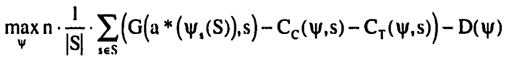
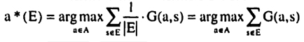
The optimization problem faced by X and Y in designing the communication protocol can be stated as follows:

This turns out to be a difficult problem to solve in general since the protocol space is both discrete and large. First, the number of possible partitions grows exponentially with the size of the state space11. Second, for most non-trivial partitions, there are several different protocols that induce the partition but have different costs.

The overall strategy for solving this optimization problem is as follows. First a simple example will be used to illustrate the problem (in Section 5.2). Second, the benefits (in Section 5.3) and costs (in Section 5.4) of bisections are analyzed in order to determine an optimal bisection (in Section 5.5). Third, the understanding of optimal bisections is used to construct optimal protocols (in Section 5,6).

11 It is easy to see that 2|S|-1 is a lower bound on the number of partitions.

5.2 Example

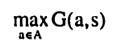
Consider the state space S = {,2,3,4,5, 6, 7,8} together with the action space A = {1,1,5, 2, 2,5,....,7,5,8}. Assume the following benefit function:

G(a, s) = 10-(a-s)2

Given the assumptions from Section 4, it is now possible to determine both the benefit and the cost of a bisection. Without any information, i.e. for the uniform distribution, the optimal action for Y is to choose a*(S) = 4.5. Doing so results in an expected benefit of

10 - l/8.(3.52+2.52+1.52+0.52+0.52+1.52+2.52+3.52) = 10 - 5.25 = 4.75

Consider the first bisection. It is easy to see that the optimal bisection for improving the expected benefit would be Ex = jl, 2,3,4} and E2 = {5,6, 7,8|. The optimal choices of actions are then a*(Ei) = 2.5 and a*(E2) = 6.5 respectively, resulting in an expected benefit of

10 - [l/2.1/4.(1.52+0.52+0.52+1.52) + l/2-l/4.(1.52+0.52+0.52+1.52)] = = 10-1.25 = 8.75

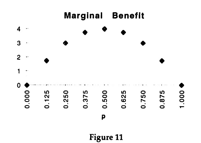
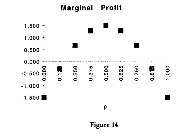
A convenient way for summarizing the possible improvements in expected benefit is to graph the marginal benefit for different probabilities of bisections. If the bisection of E is E1 and E2, let p = |E1 | / |E|. For each p several different bisections are possible, but only the one with the highest marginal benefit12 will be considered. For example, for p = 1/2 only the bisection into {1, 2,3,4} and {5,6, 7, 8} is considered instead of other bisections, such as {1, 2, 7, 8} and {3,4, 5, 6}. This method results in the following graph:

12The marginal benefit should properly be referred to as marginal expected benefit, but the "expected" is omitted for brevity.

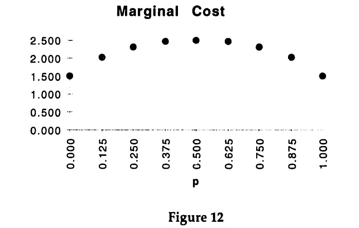
Using the assumptions about the cost of communication from above, it is also possible to determine the cost of the first bisection of the state set. Suppose that the protocol tree Ψ consists only of this first bisection, then the cost are as follows

  • D(Ψ) = d
  • Cc(Ψ, s) = cc.h(p) for all s Є S
  • CT(Ψ, s) = cT + γT for all s Є S

The cost that has to be subtracted from the benefit of the bisection for each use of the communication protocol is Cc(Ψ, s) + CT(Ψ, s).

The graph is based on assuming cT = 0.5, γT = 1.0, and cc = 1.0. The cost of design is not included and will be considered separately later on.

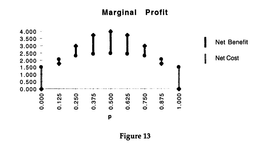
The difference between the marginal benefit and the marginal cost of using the protocol is the marginal profit.

As can be seen from Figure 13, the maximal marginal profit from the first bisection occurs for p = 0.5, i.e. when the two resulting subsets are of equal size. The optimal subsets are {1,2, 3,4} and {5,6, 7, 8}. This can also be seen by graphing the marginal profit directly, as in Figure 14.

Having determined the optimal first bisection for Example 1 raises a number of key questions that will be answered in the following sections.

Ql How can optimal bisections be determined generally?
Q2 When does the optimal bisection occur for p ≠ 0.5?
Q3 How can optimal bisections be used to describe an optimal protocol?

The answers to these questions will then be used to explain some anecdotal evidence on communication in organizations.

5.3 Marginal Benefit from a Bisection

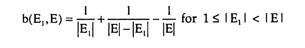
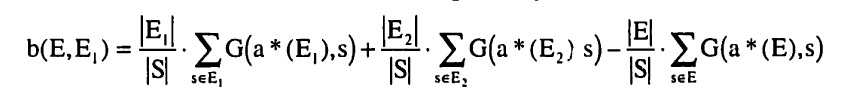
The first issue in determining an optimal bisection is to consider the marginal benefit from choosing a particular bisection. Let Ψ(S) be the partition induced by the current communication protocol. Let E Є Ψ(S) and consider a bisection of E into E1 and E2 that results in a finer partition Ψ'(S). The marginal benefit from this additional bisection is given by

The marginal benefit has a number of interesting properties which will now be examined.

Bl The marginal benefit must be non-negative, i.e. b(E, E1) ≥ 0 since choosing the optimal action a* for smaller subsets amounts to relaxing a constraint: it is always possible to choose the same action for both E1 and E2 that would have been chosen for E. The marginal benefit will also be bounded, since it is a finite sum of bounded values (given the assumption made throughout that the benefit function G(a, s) is bounded for all actions and all states).
B2 
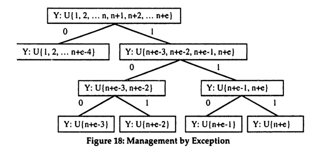
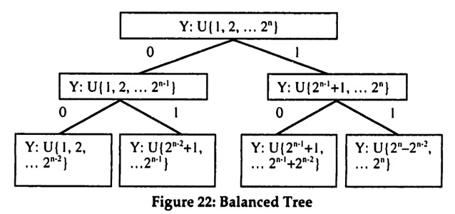
The marginal benefit can be highest for a splitting out a singleton. Consider, for instance, S = {1, 2,... n} and A = S with the benefit given by

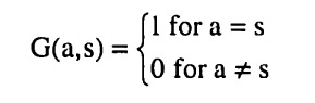
By inspection, it follows that the marginal benefits of a bisection are given by the following expression:


The expression is maximized by |E1 | = 1 and by |E1| = |E| - 1. In either case, the marginal benefit is maximal for a bisection that splits out a singleton, More generally, splitting out singletons will be optimal when the only available actions are highly specific to a particular state, i.e. have a benefit only in that state.
B3 
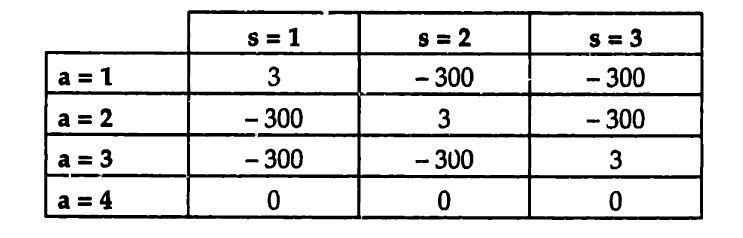
The marginal benefit from bisections can be increasing. Consider the following example where S = (1,2,3} and A = {1,2,3,4). Let the benefit be given by the following matrix:

Without any communication, the optimal action is a*{l, 2,3} = 4, resulting in an expected payoff of 0. With the first bisection it becomes possible to split out one of the states, e.g. Ψ(S) = {{1}, 12,3}}. The optimal actions are a*({l}) = 1 and a*({2,3}) = 4 and the marginal benefit is

b({l, 2,3}, {1}) = 1/3 . 3 + 2/3 . 0 - 3/3 . 0 = 1

The second bisection splits {2,3} into {2} and |3). The optimal actions are a*({2}) = 2 and a*({3}) = 3 and the marginal benefit is

b({2,3}, {2}) = 1/3 . 3 + 1/3 . 3 - 2/3 . 0 = 2

The marginal benefit for the second bisection is thus larger than the one from the first bisection. More generally, the marginal benefit is likely to be increasing when there are some specific actions that have high benefits for some specific states but do poorly in all other states, whereas other actions have moderate benefits across many states.

B4

The marginal benefit from bisections can also be decreasing. Consider the earlier example with S = (1,2,3, 4,5,6,7,8), A = (1,1.5,2,2.5 ... 7.5,8} and G(a, s) = 10 - (a - s)2. The marginal benefit from the first bisection was

b({l, 2,3,4,5,6,7,8}, {1,2,3,4}) = 8.75 - 4.75 = 4

Subsequent bisections have lower marginal benefits, e.g.

b({l, 2,3,4}, {1, 2}) = 2/8 . [10 - 0.52] + 2/8 . [10 - 0.52] -- 4/8 . [10-1/4 . (1.52 + 0.52 + 0.52 + 1.52)] = 1/2

and

b({l, 2},{1})= 1/8 .10 + 1/8 . 10 - 2/8 . [10 - 0.52] = 1/16

More generally, when there are state-specific actions, for which the benefits do not decrease too rapidly for other states, then the marginal benefit of bisections will be decreasing.

B5

The marginal benefit from bisections always drops to zero eventually. This property can be seen by considering the following definition.

Definition: A constant action subset is a subset E of S, such that one constant action a Є A is optimal for every state s Є E

It follows immediately from the definition that if E is a constant action subset then b(E, E1) = 0 for all subsets E1 of E, Hence, as soon as a partition is sufficiently fine to consist of constant action subsets only, the marginal benefit of a subsection will be zero. At the latest, a partition of all singletons will always have zero marginal benefit.13

In order to see how these properties affect the optimal protocol it is now necessary to examine the marginal cost of a bisection.

5.4 Marginal Cost of a Bisection

5.4.1 Strategy

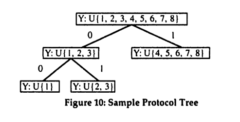
Determining the marginal cost of a bisection turns out to be more difficult than determining its marginal benefit. To understand why, consider the following example. Suppose that S = {1,2,3,4,5,6,7,8} as before. Assume that the current partition is Ψ(S) = {{1}, {2,3,4,5,6,7,8}}. What is the incremental cost of bisecting E = {2,3,4,5,6,7,8} into El = {2,3} and E2 = {4,5,6,7,8}? This is difficult since there are several possible protocols. Figure 15 and Figure 16 below show two possibilities.

13Constant action subsets will generally be larger than singletons. In fact, whenever |S| > |A|, there has to be at least one constant artion subset that is larger than a singleton. This follows because for every state there has to be at least one optimal action and if there are more states than actions, at least two states have the same optimal action.

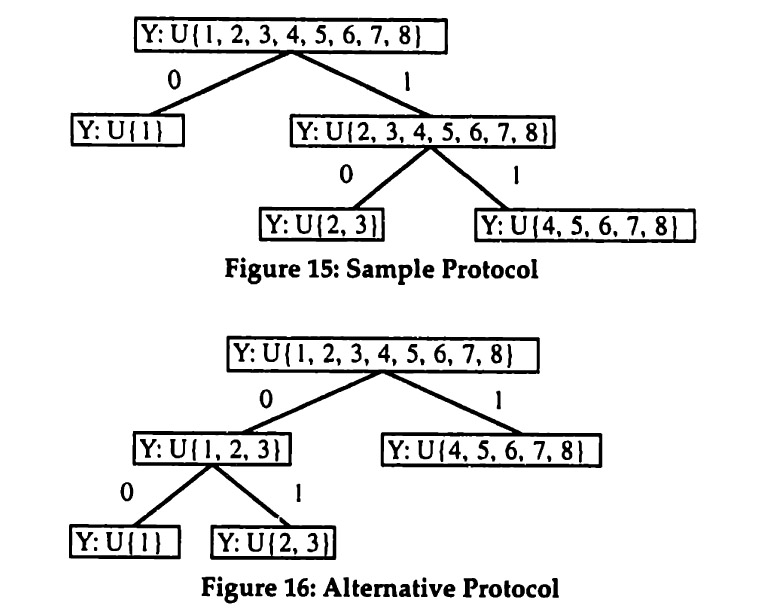
Figure 15 shows the protocol Ψ1 that would result if one took the existing protocol Ψ and extended it with the additional bisection. Figure 16 (which is a reproduction of Figure 10) shows another protocol Ψ2 that implements the same partition.

Consider the various cost components. First, the design cost is clearly the same for both protocols since both have two internal nodes. Second, the cost of coding can be calculated as follows:

E[Cc1, S)] = cc . [1 . h(l/8) + 7/8 . h(2/7)] = cc . 1.29879494
E[Cc2, S)] = cc . [1 . h(3/8) + 3/8 . h(l/3)] = cc . 1.29879494

This equality will be seen not to be a coincidence.14 Third, the cost of transmission is as follows:

E[CT1, S)] = cT . [1.1 + 7/8.2] + γT = cT . 2.75 + γT
E[CT2, S)] = cT . [1.1 + 3/8.2] + γT = cT . 1.75 + γT

Clearly, the transmission cost for protocol Ψ2 are lower than for protocol Ψ1

Hence the marginal cost of the bisection should be determined as the difference between the cost of the protocols Ψ2 and Ψ .  The strategy for determining the marginal cost of a bisection will be as follows. First, a cost minimizing protocol is developed for an arbitrary partition (Section 5.4.2).

14See Section 5.4.2 below and Appendix Al.

Second, the marginal cost of a bisection is determined as the difference in cost between two cost minimizing protocols (Section 5.4.3).

5.4.2 Least Cost Protocol

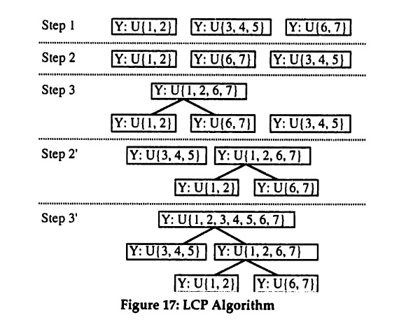
Let P(S) be an arbitrary partition of S. The objective in the first step is to find a protocol Ψ with minimal cost of communication, such that Ψ(S) = P(S).15 Consider the following algorithm for designing a protocol based on Huffman coding.16 The notation Root(Ψ) refers to the set associated with the root of the binary tree Ψ (e.g. in Figure 15, Root(Ψ) = {1,2,3,4,5,6, 7,8}).

Least-Cost Protocol (LCP) Algorithm

  1. Let each subset s ∈ P(S) be a partial binary tree Ψ, consisting of a single node, i.e. Root(Ψ) = s.
  2. Sort all partial trees according to their frequency, which is given by | Root(Ψ) |, i.e. the size of the set at their root node.
  3. Combine the two least frequent partial trees Ψ' and Ψ" into a larger tree Ψ so that Root(Ψ) = Root(Ψ') ∪ Root(Ψ").
  4. Repeat Steps 2 and 3 until there is only a single tree Ψ left.

Consider, for example, S = {1,2,3,4,5,6,7} and P(S) = {{1,2}, {3,4,5}, {6,7}}. The LCP Algorithm constructs a protocol tree as illustrated in Figure 17 below.

15This equality is a slight abuse of notation since both Ψ(S) and P(S) are sets of sets. Properly this should be written as P(S) ⊇ Ψ(S) and Ψ(S) ⊇ P(S).
16 This type of coding was introduced by Huffman (1952). For an introduction see Cormen, Leierson et al. (1990).

It will now be shown that this algorithm minimizes the cost of designing and using a protocol tree that implements the desired partition.

Proposition: Let P(S) be an arbitrary partition of S. Then the LCP
Algorithm finds the protocol Ψ which induces the partition Ψ(S) = P(S) at the minimal cost of designing and using the protocol.

Proof: First, consider the cost of protocol design. By inspection, the LCP algorithm creates a binary tree that induces the partition P(S). Since LCP creates a full binary tree,17 the number of internal nodes is minimized and is equal to | P(S) -I| The minimized cost of design is thus

D(Ψ) = d . (|P(S)|-l)

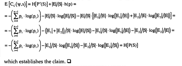
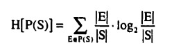
Second, consider the cost of coding. Given the assumptions, a simple inductive argument (see Appendix Al) shows that the expected cost of coding is determined entirely by P(S) for any protocol that implements P(S). Indepen­dently of the protocol structure, the expected cost of coding is

E [Cc(Ψ,s)] = cc . H[P(S)]

where H[ . ] is the entropy of the partition P(S). Given the assumption of a uniform distribution, the expression for the entropy is

17 In a full binary tree, every internal node has two children.

Third, consider the cost of transmission. As first shown by Huffman (1952), the LCP algorithm minimizes the expected path length. It hence also minimizes the cost of transmission, which is a linear function of the path length. The expected length of the path is bounded by H[P(S)] below and H[P(S)]+1 above so that the expected variable cost of transmission is

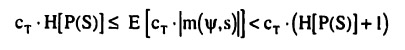
LCP thus minimizes the cost of communication.

Two results from the proof are of particular importance. First, both the cost of design and the cost of coding are seen to be independent of the protocol structure, as long as the binary tree induces the desired partition. Only the cost of transmission determines the protocol structure. Second, the proof provides expressions for the minimized cost. For the cost of transmission, however, only a range was specified since there is no closed form for the exact expected path length. For simplicity, it will be assumed that the lower bound is achieved, so that the total cost of transmission is

E[CT(Ψ,s)] = CT.H[P(S)] + γT

This assumption can be justified in two ways. First, if communication is repeated, then the lower bound is achievable as a limit by a similar algorithm (Huffman 1952). Second, the expected length is generally closer to the lower bound, except for distributions that put almost the entire weight on a few elements of the partition. In the latter case, a slight modification of the protocol—which will be discussed below (see Section 6.2)—results in an expected length close to the lower bound.

5.4.3 Marginal Cost of a Bisection

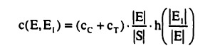
The marginal cost of a bisection can now be determined as the difference between the minimized cost for two partitions. Let P(S) be an arbitrary partition of S and let P'(S) be the partition that results from the additional bisection of E ∈ P(S) into the subsets E1, and E2. The marginal cost of design is simply the cost of adding an internal node to the protocol. Focusing on the cost of coding and the cost of transmission results in the following marginal cost.

c(E, El) = (cc + cT).{H[P'(S)]-H[P(S)]}

This expression can be simplified as follows:

The marginal cost has a number of interesting properties which will now be examined.

C1 
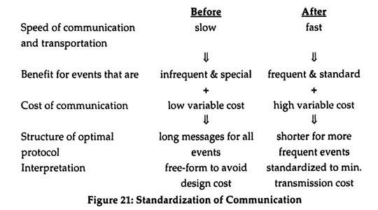
The marginal cost is strictly positive as long as cc > 0 or cT > 0. So even if communication technology were to reduce the cost of transmission to zero, the cost of coding would still result in a positive marginal cost. While the two cost components are simply additive in the expression for the marginal cost, they differ in their effect on the communication protocol. In the proof it was shown that only the cost of transmission affects the structure of the optimal protocol whereas the cost of coding was found to be constant across protocols. This difference will be seen to have implications for the effect of technology on communication protocols.
C2 The marginal cost is highest when splitting large subsets evenly. While this obviously reflects the assumptions, it also fits nicely with the intuition that the marginal cost should be highest for the highest reduction in uncertainty. As can be seen from the expression, the marginal cost is higher, if a larger subset is being bisected (the |E| / |S| term) since the cost of coding and transmission have to be incurred more frequently. The marginal cost is also higher, if the bisection is more symmetrical and hence results in a larger reduction of uncertainty (the h(.) term).
C3 The marginal cost of a bisection is decreasing. With more bisections, the size of the subsets in the partition decreases and hence the |E| / |S|term decreases towards 1/ |S| since bisections of smaller subsets are moved further down in the protocol tree by the LCP algorithm and hence occur less frequently. This property is the result of the assumption of constant marginal cost per message segment and per coding question. Clearly, these assumptions require further study. In particular, the effects of time constraints and congestion need to be explored.18
18 Time constraints, congestion of communication channels, and bounded rationality of the team members could result in increasing marginal cost for coding and transmission. This possibility is discussed in Section 7.

5.5 Optimal Bisections

Based on the marginal benefit and marginal cost of a bisection it is now possible to determine and characterize optimal bisections. An optimal bisection maximizes the marginal benefit net of marginal cost. Let E be an element of the current partition Ψ(S). Then the optimal bisection of E into E1* and E2* is determined by

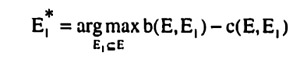
and E2* = E \ E1*. The expressions for b(E, E1) and c(E, E1) were derived in Sections 5.3 and 5.4 respectively.

These results can now be used to answer the first two questions raised at the end of Example 1 in Section 5.2:

     Ql How can optimal bisections be determined generally?
     Al Find the marginal benefit function b(E, E1) and the marginal cost function c(E, E1) and use them to determine E1* and E2*.
and

     Q2 When does the optimal bisection occur for p ≠ 0.5?
     A2 The optimal bisection occurs for p = 0.5 only for symmetric and sufficiently concave marginal benefit functions. Consider the marginal benefit function from the example used in characterization B2 (in Section 5.3), which is convex and maximal for splitting out a singleton. Given that the marginal cost function is always concave, the optimal bisection will split out a singleton.

The next section takes up the third question by examining how this knowledge of optimal bisections can be used to characterize optimal protocols.

5.6 Characterizing Optimal Protocols

5.6.1 Strategy

The understanding of the marginal benefits and costs of bisections developed above will now be used to characterize optimal protocols. The optimal protocols for the case of costly communication will be contrasted with the case of free communication. First, some weak but quite general characterizations will be given without imposing any restrictions on the benefit function (Section 5.6.3).
Second, exact optimal protocols are determined and characterized for restricted benefit functions (Section 5.6.4).

5.6.2 Free Communication

The case of free communication will be used as the benchmark for examining the effects of communication cost. It is characterized in the following proposition.

Characterization: The case of free communication, i.e. d, cc, cT, γT. = 0, has the following features

     (i)   any protocol that partitions the state set S into singletons is optimal, independent of the benefit function G(a, s);
     (ii)  it is possible for the recipient Y to choose the optimal action for every realization of the state s Є S.

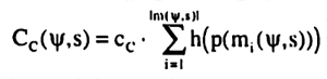
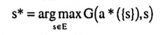
Proof: Since all protocols are costless, the team members can choose a protocol y that partitions S into singletons. After communication has taken place, the action is chosen according to

which results in the choice of the optimal action for every realization of s. It is therefore not necessary to know G(a, s) when designing the protocol. □

These features have an important interpretation: for a given state set S, the team members X and Y can design a single protocol that partitions S into singletons. This general purpose protocol can then be used by X and Y for any communication, independent of the particular decision. It is important to note that coordination on a protocol is still required, even when communication is free.19 Furthermore, a partition into singletons amounts to team member X providing Y with all the available information. Y then chooses the optimal action based on the information and carries it out. This arrangement can be interpreted as decentralized decision making, since the decision which action to choose is made by the team member who has to take the action.

19 There are many different protocols that result in a partition of all singletons and without prior agreement on one of these protocols, no communication is possible.

5.6.3 Costly Communication with General with General Benefits Functions

Based solely on the properties of the marginal benefit and marginal cost derived so far, it is possible to give a weak characterization of optimal communication protocols with costly communication.

Characterization: The case of costly communication, i.e. d, cc, cT, γT. = 0, has the following features

     (i) optimal partitions depend on the benefit function G(a, s) and never include two elements E1 and E2, such that E = E1 U E2 is a constant
action subset;
     (ii) for sufficiently high cost of communication, it may not be possible for the recipient Y to choose the optimal action for every realization of the state s Є S;
     (iii) small changes in the cost of communication can result in large changes in the amount of communication.

Proof: The marginal cost of communication is strictly positive (CI) and the marginal benefit from bisecting a constant action subset is zero (B5). Hence constant action subsets are never bisected. This establishes feature (i) since the constant action subsets are determined by the benefit function G(a, s).

There are two ways of showing feature (ii). First, since the marginal benefit is bounded (Bl), if the cost of communication is sufficiently high, then there will be no communication at all. In this case, the recipient Y has to base the choice of action solely on the prior information of a uniform distribution over the states. Except for the trivial case in which the same action is optimal for all states, Y thus cannot choose the optimal action for every realization. Second, feature (ii) also emerges when the marginal benefit of bisections declines (B4) more rapidly than the marginal cost of bisections (C3). In this case too, the optimal partition will contain elements that are not constant action subsets, hence making it impossible for Y to choose the optimal action for all realizations.

Finally feature (iii) occurs in situations where the marginal benefits of bisections are increasing (B3). Suppose that initially the marginal cost of bisections is simply too high for any communication to occur at all. Since the marginal cost of bisections is decreasing (C3), if the marginal cost ever drops below the marginal benefit, it will stay below for subsequent bisections. Hence in such a situation, as the cost of communication declines, the optimum will jump from no bisection immediately to a partition into constant action subsets. □

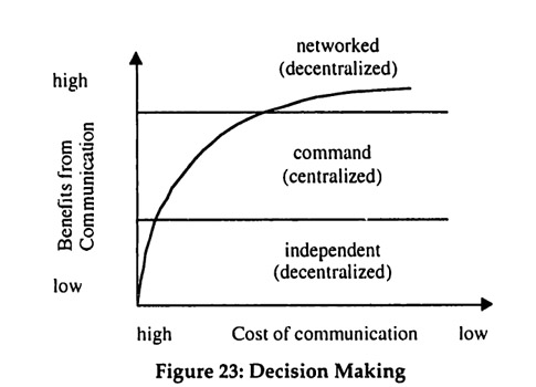
These features provide an interesting contrast with those for the case of free communication. First, with costly communication the team members can not use a general purpose protocol. Instead, different decision situations require different protocols. Second, in some situations, the optimal protocols can be interpreted as centralized decision making with the use of commands, X observes a realization of s and decides on the optimal action, which is then communicated to Y as a command. In this interpretation each constant action subset of the optimal partition corresponds to a different command, i.e. X simply tells Y which action to take. This interpretation is discussed in greater detail in one of the applications below.

5.6.4 Costly Communication with Restricted Benefit Functions

So far, the crucial third question, how optimal protocols can be constructed, has not been answered. The approach pursued here is a "greedy algorithm" (Cormen, Leierson et al, 1990). Starting with the set S, a sequence of optimal bisections is chosen one bisection at a time. Instead of looking ahead, a greedy algorithm is myopic and only optimizes the next step. The advantage of a greedy algorithm is that the characteristics of the optimal protocol follow directly from the characteristics of optimal bisections, which have been determined above.

Depending on the particular optimization problem, there may or may not exist a greedy algorithm that finds an overall optimal solution. Put differently, a sequence of optimal steps may or may not result in an optimal path. The question then is whether a sequence of optimal bisections results in an optimal protocol. Unfortunately, a greedy algorithm for general benefit functions is not possible, as counterexamples can easily be constructed (see Appendix A2 for an example)20. Instead of a general proof, the strategy therefore is to show that a greedy algorithm exists for interesting cases of benefit functions.

For a greedy algorithm to result in the optimal protocol, two properties have to hold, the Greedy Property and the Optimal Substructure Property (Cormen, Leierson et al. 1990).

20 Strictly speaking the counterexample only establishes that a greedy algorithm based on the particular metric for optimal bisections does not exist. There might be a greedy algorithm using a different metric or even a different set of steps.

     Greedy Property: For any optimal partition Ψ(S), there exists at least one sequence of bisections that results in Ψ (S) and that      starts with the optimal bisection of S.

     Optimal Substructure Property: Any subset of an optimal partition Ψ (S) is itself an optimal partition for the proper subset of S.

For a given benefit function, the challenge is to show that both properties hold. The strategy for proving the Greedy Property is quite straightforward. The proofs starts by noting that a sequence of bisections can be reordered arbitrarily and still results in the same partition. Starting with an optimal partition, it is assumed that no sequence of bisections exists results in the optimal partition and contains the optimal first bisection anywhere. This assumption is then shown to lead to a contradiction with the assumed optimality of the sequence. The Optimal Substructure Property amounts to a regularity condition on the benefit function. The available actions and the structure of the benefits has to be similar for subsets of the states. In the examples considered below, the Optimal Substructure Property will follow immediately from the restrictions on the benefit function.

Suppose now that the two properties have been shown to hold for a particular benefit function. The characteristics of the optimal protocol can then be derived from the characteristics of an optimal bisection, which answers the third question raised in Section 5.2:

     Q3 How can optimal bisections be used to describe an optimal protocol?
     A3 If the greedy property and the optimal substructure property hold, a sequence of optimal bisections will result in an optimal      protocol.

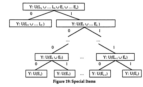
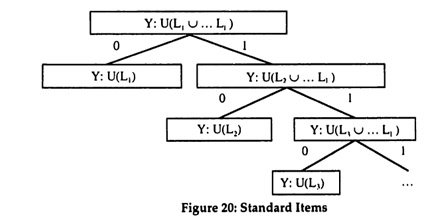
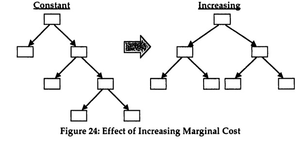
For example, if the optimal bisection splits out a single state, then as the cost of communication drops, the optimal protocol will consist of an increasing number of individually identified states. The discussion of anecdotal evidence in the next section contains concrete examples of benefit functions for which both properties hold.

6. ANECDOTAL EVIDENCE

6.1 Caveat

The analysis of communication based on the properties of finite protocols as proposed above is novel and this paper is only a first step. The purpose of the following examples of anecdotal evidence is therefore mostly to illustrate that this approach holds promise, rather than to provide an in-depth analysis of any particular phenomenon. With this in mind, the examples considered are management by exception, standardization of communication, and decentralization of decision making.

6.2 Management by Exception

A common technique for reducing the information processing load of managers is known as "Management by Exception" (MBE). With MBE, information is only communicated to the manager (Y) by an employee (X) when an exception has occurred which requires an action by the manager. The protocol-based approach will now be used to provide a fundamental explanation for this phenomenon.

Assume that the set of states S consists of the two subsets N = {1, 2,... n| for normal states and E = {n+1, n+2,... n+e} for exception states, with n > e. For each exception, i.e., for each state s Є E, there is exactly one optimal action a*({s}) by the manager, such that
     G(a*({s}), s} » 0
and
     G(a*({s}), s') « 0 for s' ≠ s

In words, the optimal action for an exception has a high benefit when that exception occurs, but should not be chosen in any other state.21 For all normal states, the manager's actions have no benefits

     G(a, s) = 0 for ∀a Є A if s Є N

Finally, there is a constant action á Є A that the manager can always choose such that

     G(á, s) = 0 for ∀s Є S

The action á will be interpreted as the manager "doing nothing," i.e. not taking any other action.

It is easy to see that the optimal first bisection is to split out the exception state s* with the highest benefit from managerial intervention, i.e.

21 Given the assumption of uniform distributions, this setup amounts to assuming that all exceptions are equally likely. The example can easily be generalized to allow for different likelihoods.

The Optimal Substructure Property follows immediately from the assumptions. Due to the regularity of the benefits, any subset of states has a benefit structure that is similar to the overall set. The Greedy Property can be shown as follows. Let Ψ*(S) be an optimal non-trivial partition.22 Assume that there is no sequence of bisections that splits out s* and results in Ψ*(S). But the net benefit from any sequence that does not split out s* can be improved by replacing an arbitrary bisection with splitting out s* and hence Ψ*(S) could not have been optimal. This follows because the marginal cost of splitting out a single state was shown in Section 5.4 to be lowest and the marginal benefit from splitting out s* is highest by assumption.

Given that the two properties for a greedy algorithm hold, it is easy to characterize the partition resulting from the optimal protocol based on the optimal bisections. The optimal partition splits out exception states in order of the benefit from managerial action. As the cost of communication drops, more exception states are split out until eventually every state in the subset E is individually identified. For each exception state that has been split out, the manager takes the optimal action. For all other states, the manager does nothing. The actual structure of the communication protocol now follows directly from applying the LCP to the optimal partition and is shown in Figure 18. In constructing Figure 18, it was assumed without loss of generality that the exception states are ordered by the benefit from managerial action, i.e. the benefit is greater for state n+2 than for state n+1 and so on. Furthermore, the cost of communication was assumed to be sufficiently high that only four exception states were split out.

22 A non-trivial partition has at least two subsets, i.e. is the result of at least one bisection.

Given the original assumption that n > e, i.e. there are more normal states than there are exception states, the optimal protocol frequently results in a single "0" being sent.23 In this case the manager updates the available information to U{1,2,... n+e-i} (where i S e), which means that the manager is forced to do nothing. Even though for i < e an exception state may have occurred, the manager does not know which state it was and hence cannot take an action.

In this type of highly unbalanced protocol, where one path occurs much more frequently than all others, the cost of transmission is close to the upper bound (see Section 5.4.2). Suppose now that the communication channel has the special property that it is reliable, so that any message that has been sent by the employee is always received by the manager. In this case, the cost of transmission can be reduced to the lower bound by not sending a message at all if and only if the message would have been a single "0".24 This is effectively MBE, i.e. a message is sent to the manager only when an exception state has occurred and hence the manager has to take an action. In addition to reducing the expected message length, MBE also eliminates the fixed cost of transmission and reduces the cost of coding for all normal states.

23 Note that n > e is necessary for the normal subset to be discriminated by the first bisection in the protocol, as can easily be seen by inspection of the LCP algorithm.
24 At first this may appear like a "slight of hand" that violates the idea of a binary protocol. In particular, one might ask why this option is not available at each level and thus permit trisections instead of bisections. The answer is that a communication channel first has to be activated (hence the fixed cost of transmission). Once it is activated, not sending is not an option, since it effectively amounts to the termination of communication.

This fundamental explanation of MBE provides several interesting insights. The driver behind MBE is that it economizes on communication cost by reducing the expected variable cost of transmission and eliminating the fixed cost of transmission and the cost of coding for all normal states. But MBE in turn requires a reliable communication channel. In a broad interpretation, the reliability of the channel includes the proper incentives for the employee to send a message whenever one is required, i.e. to report exceptions. It is easy to see that this may not always be the case (e.g. the exceptions might be the results of errors by the employee). Hence, the applicability of MBE may be restricted by incentive reasons, even when it is desirable in principle.

Improved information and communication technology will affect the desirability and applicability of MBE. Obviously, if communication cost were completely eliminated, there would be no reason for MBE. Instead a more common scenario is that the cost of encoding a state (e.g. the daily sales of a store in a chain of stores) and transmitting a message has been essentially eliminated, but not the manager's cost of decoding. In this case, MBE will take the form of an Executive Information System (EIS), where information is collected automatically from all employees, but the EIS notifies the manager only when there is an exception. To the extent that the automatic collection eliminates the incentive constraints on the reliability of the communication channel, one should expect to see an increase in the use of MBE supported by EIS, which is consistent with the available anecdotal evidence.

6.3 Standardization of Communication

Yates (1989) argues that the standardization of business communication was a key innovation in the development of the modern industrial enterprise. The time period which she studies was marked by revolutionary technological advances in two areas: the telegraph in communication and the railroad in transportation. The protocol-based approach will now be used to show that the standardization of communication can be seen as a logical response to these technological advances rather than a separate innovation.

The communication between a store (X) and a manufacturer (Y) will serve as an example. The store observes a small number of frequent events (e.g. the stock of a standard item running low) and a large number of infrequent events (e.g. requests for special items). This will be represented by a set of states S consisting of two classes of subsets: a few large subsets L1…1 and a large number of small subsets E1…e, i.e. | Li| » | Ej | and 1« e. All subsets are constant action subsets (see Section 5,3), i.e. there is a single action that is optimal for the entire subset. The benefits are assumed to be as follows:

G(a*(Li),s) = GL if s Є Li and G(a*(Li),s) = 0 if s Є Li

G(a*(Ei),s) = GL if s Є E i and G(a*(Ei),s) = 0 if s Є E i

Put differently, for each event there is exactly one beneficial action by the manufacturer (e.g. supply the appropriate item). The constant benefits are for simplicity and can be thought of as constant profit margins. 25

Consider first the situation prior to the telegraph and the railroad. The communication between the store and the manufacturer is by written letter and the transport of goods by horse-drawn wagon. There is little benefit from communicating when the stock of a standard item is running low since the combined time for communication and delivery is long. Instead, traveling sales agents or manufacturer representatives come around periodically to offer the standard items for replenishment. This implies GL = 0, which leaves requests for special items. Assuming that the waiting time is acceptable foi special items, i.e. GE > 0, the situation is similar to Management by Exception (in Section 6.2) and results in the optimal protocol shown in Figure 19.

25 The benefits in the example can be generalized. While adding realism, such increased richness makes the key insights harder to discern.

At the time, the cost of transmission for a letter were low (especially the variable cost, see Appendix A3) and so were the coding cost (due to cheap labor). Therefore, given that the number of different special items is large, the right side of the protocol tree in Figure 19 is deep for each special order. But this raises the issue of the cost of protocol design: agreeing on all the questions in advance may be prohibitive. The logical alternative to structured communication are free form letters. Instead of designing a protocol, i.e. agreeing on a set of questions and transmitting only the answers, a free form letter contains both the questions and the answers.

Now consider the situation after the advent of the railroad and the telegraph. The combined communication and transportation time is cut dramatically. Instead of waiting for an agent or representative to come around, there is now a benefit from ordering the replenishment of standard items via telegraph when these are running low, so that GL > 0. The use of a public telegraph generally had high variable cost, since there was a charge for every ten words in a telegram (see Appendix A3). Ignoring for the moment the special items, the optimal protocol for replenishment was therefore likely to be structured as in Figure 20.

The underlying assumption for the structure in Figure 20 is that some standard items need to be restocked more frequently than others.26 It is then straight-forward to verify that both the optimal substructure and the greedy properties hold.27

The key feature of the optimal protocol is that frequently occurring events result in the shortest messages. The literal interpretation is that those standard items which need to be restocked more frequently receive shorter descriptions. A slightly more liberal interpretation is that all standard items have the same code length, but the store only includes those standard items in the message that actually need to be restocked. The events are then the number of different standard items that need to be restocked on a particular day.28 In either interpretation, the communication is highly standardized. For the communication of orders for special items, the arguments from above still apply. It is therefore likely that free-form letters will continue to be used to order special items.

The simultaneous change in communication and transportation technology thus results in the introduction of standardization as an optimal protocol. In this view, standardization of communication is a rational behavior change in response to technological innovation.

26 It was assumed, without loss of generality, that the subsets are ordered by decreasing size, i.e. |L1| > |L2| and so on, which implies decreasing frequency of the need to restock.
27An additional condition for the optimal protocol to have the structure shown in Figure 20 is that GL is sufficiently big to make the optimal first bisection split out the largest (rather than the smallest) subset.
28As long as the likelihood of any standard item needing to be restocked is sufficiently small, the resulting distribution will be such that days with few items needing to be restocked are more frequent.

The argument is summarized in Figure 21. While the example of a store and a manufacturer were used for illustration, the logic of the argument is quite general. Increased standardization essentially only requires two conditions to hold: first, more frequently occurring events have to require faster action in order to obtain a benefit and second, the new and faster form of communication has higher variable cost of transmission. As was shown above, the historic evidence suggests that both conditions held at the time of the introduction of the telegraph. During this time period, standardization was also favored by a shift in production technology from craft production, which could easily accommodate special orders, to mass production, which focused on driving down cost for a small set of standard orders. Thus the percentage of communication dealing with standard orders was increasing relative to that dealing with special orders.

The trend towards standardization was later reinforced by the emerging use of computers in business. The cost of storage is exactly analogous to the cost of transmission. Longer messages require more computer memory and hence incur higher storage costs. With today's affordable personal computers that have many megabytes of storage, it is easily forgotten that early mainframe computers - which only the largest corporations could afford - had only a few kilobytes of memory. Put differently, there has been a tremendous reduction in the price per byte of storage, where today the variable cost of storage is essential zero.29 It is therefore not surprising that computers initially were used to store highly structured information only (e.g. accounting data), whereas today computers store large amounts of unstructured information (e.g. correspondence).

The reversal of the standardization trend is not only the result of cheaper computer storage. Standard communication is increasingly being automated (e.g. sales and production reports) and a shift from mass production to modular production, as well as the decline of manufacturing relative to more customization-oriented service industries, are contributing to a decrease in the relative importance of standardized communication.

29 There are still capacity constraints, i.e, while each byte is more or less free, when the capacity of memory is exhausted there are high marginal cost. The implications of capacity constraints are discussed in Section 7.

6.4 Decentralization of Decision Making

6.4.1 Background

Historical case studies on the emergence of the modern enterprise (e.g. Chandler 1977) provide evidence that improvements in communication technology were accompanied by increased centralization of decision making and the use of commands. Manufacturers integrated forward into distribution and sales representatives who had previously worked on commission became salaried employees. Recently, further improvements in communication technology appear to be related to the opposite trend, i.e. the increased decentralization of decision making. For instance, Brynjolfsson and Hitt (1996) find in a study of large firms that increased use of computer networks is associated with decentralization and incentive pay. There thus appears to be a pattern of initial centralization followed by decentralization, which will now be explored using the protocol-based approach.30

6.4.2 Setup and Protocol Structure

Consider the communication from a central office (X) to a local agent (Y).31 The state space will be a generalized version of the example introduced in Section 5.2, i.e. S = {1,2,... 2n}, together with the appropriate action space A = {1, 1.5, 2, 2.5,... 2n-0.5, 2n|. The benefit function is given by

G(a, s) = G- (a-s)2

for a sufficiently large constant G. Based on the example, the optimal first bisection splits S into two equal halves. The Optimal Substructure Property follows immediately from the assumptions. The Greedy Property can easily be shown to hold. Let Ψ*(S) be an optimal non-trivial partition. Assume that there is no sequence of bisections that splits S evenly and results in Ψ *(S). This means that every sequence that results in Ψ *(S) contains at least one bisection of a subset E of S into E1 and E2 such that | | E1 | - |E2||≥ 2, Replacing these with E1' and E2', such that E1' U E2' = E and | |E1' | - |E2' || ≤ 1 results in a new partition Ψ'(S). Let B(-) and C(-) denote the total benefit and cost of a protocol respectively, then

30 See Malone and Wyner (1996) for a related analysis of this phenomenon.
31 Note that the direction of communication here is "opposite" to the previous two applications which were from an employee (local) to a manager (central) and from a store (local) to a manufacturer (central).

B(Ψ')-C(Ψ ') =
= B(Ψ) - b(E, E1) + b(E, E1') - [C(Ψ) - c(E, E1) + c(E, E1’)] =
= B(Ψ) - C(Ψ) + [b(E, E1’) - c(E, E1’)] - [b(E, E1) - c(E, E1)] >
 > B(Ψ) - C(Ψ)

The inequality follows since given the assumptions a more even split of any set has a higher net benefit (see Section 5.2 for illustration).

Given that both the Optimal Substructure Property and the Greedy Property hold, the structure of the optimal protocol is as shown in Figure 22.

The protocol tree will always be balanced32 since the net benefit of splitting a set is identical for all sets of the same size. The optimal partition thus consists of equal sized sets.

The optimal protocol in this example differs crucially from the ones in the two preceding sections. Unlike before, the sets that are split out are not constant action subsets. Unless the communication cost is so low that the optimal partition contains only singletons, the information communicated to the local agent has a "lower resolution" than the information available to the central office. This fact will be used to provide a possible explanation for the observed pattern of initial centralization and subsequent decentralization with improved communication technology.

6.4.3 Bare Bones Analysis of the Centralization-Decentralization Pattern

Consider starting with the cost of communication so high that even the first bisection does not have a net benefit. In that case, it is obvious that no communication will take place and effectively the local agent acts independently from the central office based only on the prior knowledge of the uniform distribution over 5. The optimal choice of action is a*(S) = 2n-1 + 0.5. As the cost of communication drops, there will eventually be a benefit from bisecting S into E1 = {1, 2,..., 2n-1} and E2 = {2n-l,... 2n}. The optimal choices of actions are a1* = a*(E1) = 2n-2+0.5 and a2* = a*(E2) = 2n-1 + 2n-2 + 0.5.

Therefore, if the central office (X) sends a 0 (see Figure 22) this can be interpreted as a command to the local agent (Y) to perform the action a1* and similarly a 1 is a command to perform a2*. The interpretation of the message segments as commands is based on two characteristics of the protocol. First, the local agent receives only a small fraction of the information available to the central office. Second, the agent does not need to know the benefit function and does not have to carry out an independent choice. All the agent needs to know is that 0 requires performing a1* and 1 requires a2*.

As the cost of communication drops further, more and more bisections become possible. As the partition induced by the protocol becomes increasingly fine, there is a gradual change in the nature of communication. Instead of many different commands, the longer messages become more and more like the provision of information to an agent. Instead of the agent having to remember what each command means, the agent may instead be trained to understand the benefit function and choose the optimal action based on the partial information provided by the center. This latter interpretation is strongest once the cost of communication has dropped far enough for the optimal protocol to partition S in to singletons.

While this bare bones analysis establishes the basic pattern of centralization and decentralization, it lacks many organizational details, such as incentives. In particular, the changing interpretation of messages from commands to partial information can be attacked as arbitrary. After all, even the single 0 and 1 could be interpreted as providing the local agent with partial information, albeit particularly crude. The next section shows that by adding incentives and local information, the differences between centralization and decentralization can be made more realistic.

6.4.4 In Depth Analysis of the Centralization-Decentralization Pattern

In general, the correct choice of action will not only depend on the central information, but also on information available to the local agent. To avoid having to model bi-directional communication, it will be assumed that the local information is revealed to the agent at the last possible moment, so that there is no opportunity for communicating the local information to the central office prior to having to choose the action. Another factor influencing the benefit in a more realistic setting are the agent's incentives to carry out the correct action.33 Even when the agent has all the information available, without proper incentives, the agent may not choose the right action.

Assume that the local agent observes a binary state 1 Є {Up, Down} and takes a two-dimensional action, where one dimension is from the action set A and the other dimension is b Є {Up, Down, do nothing}. When the agent's action b matches the local information I this results in an additional fixed benefit K for the agent. The agent thus has an incentive to react to the local information. But if the agent chooses "Up" when the central state s is an even number, then there is a cost for the central office. Thus half the time the agent's reaction to the local information is not desirable from the perspective of the central office.

A concrete example will help motivate these stylized assumptions. Suppose that the local agent is a sales agent and that the central office has information about the profitability of two different product lines A and B sold by the agent. This profitability varies according to factors observed only by the central office, such as capacity utilization, input prices, and strategic direction. The sales agent, on the other hand, observes whether a particular customer can more easily be convinced to buy product A or product B. An easy sale gives the sales agent the private benefit of having to exert less effort. Allowing the sales agent to react to this local information will have a cost for the central office, if the agent sells the less profitable product.

Given the assumptions, the optimal arrangement is summarized in Figure 23. The shape of the benefits from communication is the result of declining marginal benefits, which were demonstrated for this setting in Section 5.3 (B4).

33 See Section 7 for a discussion of bi-directional communication.

Each of the three areas in Figure 23 and the transitions between them will now be described in detail.

  • Independent
    When the cost of communication is high, the optimal message resolution is coarse and hence the achievable benefits from choosing an action from set A are low. At the same time, the coarse information also means that the agent has to be prevented from matching the b action against the local information in order to avoid costs for the central office. This incurs a fixed cost of K, e.g. by making the agent an employee and paying a fixed salary.34 As long as K exceeds the achievable benefits, it will be optimal to have no communication and let the local agent make all decisions. In this case the agent will choose a*(S) = 2n-1 + 0.5 along the first action dimension and will match the second action dimension to the local information. The agent thus operates independently and no communication takes place.
  • Command
    As the cost of communication declines, the optimal message resolution increases and so do the achievable benefits from communication. Eventually the fixed cost K is exceeded and the agent is made an employee with a total compensation of at least K. The employee effectively receives commands from the central office which action from A to choose. Through job design,monitoring, and monetary incentives the employee is prevented from matching the second action dimension and instead chooses to "do nothing" for action b. These are "narrow" incentives that are aimed at ensuring that the employee carries out the commands and does not react to the local information.
  • Networked
    As the cost of communication declines further, the optimal message resolution continues to increase. At some point, it is sufficiently fine for the local agent to decide when matching the second dimension is possible without incurring a cost for the central office.35 Now it is once again optimal to let decisions be made locally. A new incentive structure is required so that the agent will react to the local information when there is no cost to the central office but not otherwise. Such an arrangement can be seen in some of the emerging networked organization structures, which provide "broad" incentives that balance local with central payoffs.
34 Some amount of monitoring or job design will be required to prevent the agent from gaining the additional benefit even after receiving the wage. The bottom line is a minimal cost of K, since this is the agent's outside option.
35 Given the assumptions, this requires that the cost of communication are so low that the optimal partition consists of singletons.

As the cost of communication falls, there is thus initially centralization, as the local agent shifts from being independent to being an employee that follows commands. Subsequently, as the cost of communication falls further, there is decentralization as the employee once again becomes the decision maker.

For the example of sales agents, there is substantial historical and anecdotal evidence to support this analysis. For instance, Chandler (1977) has documented the transition from independent sales agents to employed sales personnel that occurred as communication cost was reduced due to the increasingly widespread use of the telegraph. The independent sales agents frequently had market incentives since they took ownership of the goods. They also decided which selection of goods to sell. The employed sales personnel differed substantially. While they may have had strong sales incentives, these were narrowly geared to the particular products that they were selling and they had no or only very limited choice of which products to sell. This essentially remained the arrangement for most sales personnel until relatively recently. With the introduction of so-called "sales force automation" software, sales agents can be provided with online information about the availability and profitability of a large number of products. Instead of narrow incentives which steer the agents towards one or the other product, agents are increasingly being provided with broad incentives (e.g. the overall profitability of a particular customer or segment). The sales agents are given much broader decision rights, including which products to sell, which may also include products from partner firms in order to form a complete solution for a customer.

7. CONCLUSION

7.1 Contributions

This paper started by stating the need for an improved theoretical understanding of the cost of communication and pointing out a gap in the existing literature. It then proposed an approach based on optimal finite protocols to fill this gap. In order to implement the protocol-based approach, a variety of assumptions for assigning costs and benefits to protocols were introduced. Based on these assumptions, the characteristics of optimal protocols were derived by breaking the optimization problem up into a series of small steps. First, the marginal benefits and costs of a bisection36 were analyzed. The marginal benefits and costs were then used to determine an optimal bisection. Finally, a sequence of optimal bisections was used to characterize the optimal protocol.

The results were used to contrast optimal protocols for costly communication with the case of free communication. It was shown quite generally that costly communication necessitates the use of special purpose protocols. These protocols, which can sometimes be interpreted as commands, may not provide enough information for the recipient to choose the optimal action. Furthermore, it was demonstrated how a small change in the cost of communication can result in a large change in the amount of communication.

In addition to these general results, the protocol-based approach was used to examine some anecdotal evidence about communication in organizations. First, a fundamental explanation for Management by Exception was provided based on savings in communication cost. Second, the historic standardization of organizational communication was interpreted as an adaptation of optimal protocols to the dramatic improvements in communication and transportation brought about by the telegraph and railroad. Third, it was shown how a pattern of centralization and decentralization of decision making may result from improvements in communication technology.

36 A bisection is a one-step extension of a protocol, See Section 3.4 for a definition.

7.2 Next Steps

7.2.1 Overview

The results in this paper are clearly only a first step. They do, however, indicate that the protocol-based approach for studying communication is worth pursuing further. Throughout the paper, a number of obvious next steps were pointed out. Two of these will now be discussed in greater detail. First, the effects of time constraints, congestion of communication channels, and bounded rationality on optimal protocols will be discussed (Section 7.2.2). Second, it is shown how the protocol approach can be extended to the case of bi-directional communication (Section 7.2.3).

7.2.2 Increasing Marginal Cost

In Section 4 it was assumed that the marginal cost of coding (cc) and the marginal cost of transmission (cT) are both constant. There are situations in which these assumptions do not hold. For instance, when communication channels are time or capacity constrained or are congested, the marginal cost of transmission may suddenly increase substantially and may even become infinite (e.g. if a channel is available only for a certain time period). Similarly, with bounded rationality, team members may experience increasing marginal cost of coding. There are likely to be situations when there are time and capacity constraints on the ability to code, which in the extreme may result in infinite cost of coding.

The effect of increasing marginal cost of coding and transmission on optimal protocols is the same: longer paths become relatively more expensive and hence protocol trees will be more balanced than they would be otherwise, as shown in Figure 24. Trees that are already balanced will be less deep and hence provide less information. This effect has interesting implications for each of the three examples of anecdotal evidence discussed in Section 6:

  • Management By Exception (MBE)
    Balancing the tree in the case of MBE can be interpreted as "over-flowing" the reporting of past exceptions to a time when no exception has occurred. If such "over-flowing" frequently becomes necessary, it may instead be optimal to report at set intervals. These types of "standing" meetings are in fact common in situations with time constraints, such as software development projects on tight deadlines.
  • Standardization of Communication
    In the context of standardization, a direct interpretation of more balanced protocol trees are numerical codes, which force messages of varying lengths are forced into the same length. For instance, instead of product names, it is common to transmit orders using numeric product codes. Messages may be further shortened by omitting segments which rarely change. The best-known example of this is of course the Year 2000 Problem (frequently referred to as "Y2K") which results from the fact that many computer programs in order to economize on "message" length for storage purposes, stored only the last two digits of a year.
  • Decentralization of Decision Making
    In the setup used in Section 6.4 to analyze changes in the location of decision making, the protocol tree was already balanced. Increasing marginal cost would then result in a tree that is less deep and hence provides less information, which implies that the independent or command arrangements are becoming relatively more likely. This implication is consistent with the observation that in times of crises when communication channels tend to be overloaded, the command mode, or in the extreme independent decision making tend to be prevalent.

These results, while clearly preliminary, are encouraging. They show that the initial assumption of constant marginal cost constitutes a valid base case that can then be adapted to other conditions.

7.2.3 Bi-Directional Communication

Another huge simplification made throughout the paper was the assumption that information needs to be communicated in one direction only. In most settings, information is distributed across many locations and hence communication has to be at least bi-directional. The protocol-based approach can be extended to take this into account. This sections uses a simple example to illustrate how such an extension can be accomplished and some of the insights it is likely to provide.

Let the state space be given by S = Sx \otimes \!\, 
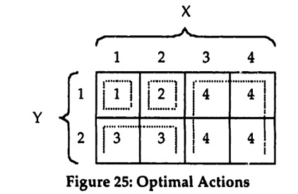
SY, where Sx = {1, 2,3,4} and SY = {1,2}. This two dimensional state space represents the information observed by the two team members X and Y. Let the set of actions be given by A = {1,2,3,4}. Finally, to keep the example really simple, assume that the benefit function is represented by the matrix in Figure 25, where the action shown for each cell has a benefit of 1 in that cell and all other actions have no benefit. It follows immediately that Figure 25 shows the optimal action for each possible state.

Also shown in Figure 25 are constant action subsets for each of the optimal actions, as indicated by the dotted lines. Since a communication protocol will again consist of bisections, it follows by induction that only "rectangles" are well-formed constant action subsets, where a rectangle is given by Ex \otimes \!\, EY where Ex is a subset of Sx and EY of SY respectively. 37

Cost minimizing protocols can again be determined by an approach similar to that introduced in Section 5 above. In this simple example, it will further be assumed that the cost of communication is sufficiently low that a partition into the indicated constant action subsets is possible. The focus will be on the cost-minimizing protocol. Building the protocol "bottom-up" by starting with the constant action subsets and combining subsequently larger sub-trees results in the protocol show in Figure 26.

37 Note that a rectangle does not have to be a geographic rectangle in diagrams like Figure 25, since columns and rows do not need to be adjacent.

The optimal protocol constructed this way has the feature that the communication alternates between the two team members X and Y. This can be interpreted as synchronous communication, which requires both parties to simultaneously participate in the communication. Given the assumed uniform distribution, it can be seen by inspection that the expected message length is (8/8) • 1 + (4/8) • 2 + (2/8) • 3 = 22/8 = 2.75.

Figure 27 shows an alternative asynchronous protocol, where team member Y starts by sending the available information and team member X responds at some later point.

Again, the expected total message length for the asynchronous protocol from Figure 27, can be determined by inspection as (2/2) • 1 + (4/4) • 1 + (2/4) • 2 = 3. The asynchronous protocol thus has a higher cost of communication than the optimal protocol determined using the "bottom-up" construction approach.

The example obviously only scratches the surface of bi-directional communication. Nevertheless, it serves to illustrate the additional complexity that results from having distributed information. While the key difficulty lies again in simultaneously determining the benefit and the cost of different protocols and optimizing over the space of all protocols, this turns out to be significantly more difficult in the two dimensional case.

7.3 Outlook

An ideal goal for further research is to use the protocol-based approach to derive simplified models of communication cost that are nevertheless grounded in fundamentals. Much like Holmstrom and Milgrom's paper on "Aggregation and Linearity" (1987) paved the way for studying a large number of incentive problems using simple linear schemes, such a result would greatly contribute to the exploration of communication problems.

APPENDIX

A1. Cost of Coding

Claim: For any partition P(S), the cost of coding is independent of the structure of the protocol and is given by

E [Cc(m(x,Ψ), Ψ)] = cc • H [P(S)]

where H[ • ] is the entropy of the partition P(S).

Proof: By induction on | P(S) |. Assume without loss of generality that cc = 1 to simplify notation. Base case: | P(S) | = 1. If P(S) has only one element, it must be S, so H[P(S)] = 1 • log 1 = 0. This is the correct cost, since no coding is required and hence the claim is true for the base case. Inductive hypothesis: |P(S) | = n. Assume the claim is true when P(S) has n elements. Induction: | P(S) | = n + 1. Consider the binary tree Ψ for a protocol that implements P(S) and assume without loss of generality that Ψ is a full binary tree, i.e. each non-terminal node has two children (any nodes with only one child can be eliminated). Find a non-terminal node N so that both children of N are terminal nodes. A full binary tree is guaranteed to have at least one such node. Denote the elements of the partition P(S) at the two terminal nodes as E1 and E2. Let E = E1 U E2. Let p = |E1 | / |E|. Then the cost of coding incurred at N is h(p). Now, consider the tree Ψ' where N is replaced by a terminal node with the subset E, so that implements P'(S) which has n elements. Using the inductive hypothesis, it follows that E[CC(Ψ', s)] = H[P'(S)]. The expected cost of coding for y can now be derived as follows:

A2. Counterexample for Greedy Algorithm

Consider the following matrix of benefits for various combinations of states and actions.

  s = l s = 2 s = 3 s = 4
a = l 3 -1000 -1000 -1000
a = 2 1 1 -1000 -1000
a = 3 -1000 -1000 2 -1000
a = 4 -1000 -1000 -1000 2
a = 5 0 0 0 0

Assume further that the cost of communication are non-zero but sufficiently low to allow for at least two bisections.

The following table lists the benefits from all possible first bisections (these can easily be derived by inspection).

E1 E2 Benefit
{1} {2,3,4} 3/4
{2} {1,3,4} 1/4
{3} {1,2,4} 2/4 = 1/2
{4} {1,2,3} 2/4 = 1/2
{1,2} {3,4} 1/4 + 1/4 = 1/2
{1,3} {2,4} 0/4 = 0
{1,4} {2,3} 0/4 = 0

The optimal first bisection is clearly E1 = {1} and E2 = {2,3,4}, since it has the highest marginal benefit and the lowest marginal cost.
Now consider the marginal benefits from a second bisection, given that the optimal first bisection was chosen.

E1' E2' Benefit
{2} {3,4} 1/4
{3} {2,4} 2/4 = 1/2
{4} {2,3} 2/4 = 1/2

Hence the maximal total benefit after having chosen the optimal first bisection is 3/4 + 1/2 = 5/4. Contrast this with the total benefit from the partition {{1, 2}, {3}, {4}}, which can easily be verified to be 6/4. Since this partition can only be achieved by choosing a sub-optimal first bisection, it follows immediately that a greedy algorithm based on the optimal bisection as defined here cannot be successful.

A3. Historical Cost of Communication

Based on the Historical Statistics of the United States (1976), the rates for letters in 1908 were 2 cents per 1/2 oz., independent of distance within the 50 states. A 1/2 oz. letter can contain three to four pages of paper, which with average handwriting or single-spaced typing can hold upward of 1,500 words. The cost of transmission is thus essentially fixed and extremely low. Telegrams on the other hand were restricted to ten words or fewer. In 1908 the rate for a telegram from New York City to Chicago was 50 cents and to San Francisco it was 100 cents. The restriction to ten or fewer words means that the cost of transmission is effectively variable with an average rate of 5 to 10 cents per word. In 1908 the telephone was a possible alternative to letters and telegrams, but it was not yet in widespread use. Its adoption had been slowed down by high rates for the installation and rental of handsets, as well as the high long distance usage rates.

REFERENCES

Brynjolfsson, E. and L. Hitt (1996). "IT and Organizational Architecture." mimeo.
Chandler, A. D. J. (1977). The Visible Hand. Cambridge, Massachusetts, Harvard University Press.
Cormen, T. H., C. E. Leierson, et al. (1990). Introduction to Algorithms. Cambridge, The MIT Press.
Green, J. and J.-J. Laffont (1986). Incentive theory with data compression.
Uncertainty, information, and communication. W. P. Heller, R. M. Starr and D. A. Starrett Cambridge, Cambridge University press: 239-253.
Green, J. and J.-J. Laffont (1987). Limited Communication and Incentive
Compatibility. Information, Incentives, and Economic Mechanisms. T. Groves, R. Radner and S. Reiter, Minneapolis, University of Minnesota Press: 308-329.
Historical Statistics of the United States (1976). Bicentennial edition, published by the U.S. Department of Commerce, Bureau of the Census. Washington, D.C.
Holmstrom, B. and P. Milgrom (1987). "Aggregation and Linearity in the Provision of Intertemporal Incentives." Econometrica 55(2): 303-28.
Huffman, D, A. (1952). "A Method for the Construction of Minimum-Redundancy Codes." Proceedings IRE 40(9 (Sept.)): 1098-1101.
Hurwicz, L. (1986). On informational decentralization and effiency in resource allocation mechanisms. Studies in Mathematical Economics. S, Reiter. Providence, The Mathematical Association of America.
Kreps, D. M. (1990). A Course in Microeconomic Theory. Princeton, Princeton University Press.
Malone, T. and S. Smith (1988). "Modeling the Performance of Organizational Structures." Operations Research 36(3): 421-436.
Malone, T. and G. Wyner (1996). "Control, Empowerment, and Information Technology." mimeo.
Marschak, J. and R. Radner (1972). Economic Theory of Teams. New Haven, Yale University Press.
McLuhan, M. (1962). The Gutenberg Galaxy: The Making of Typographic Man. Toronto, University of Toronto Press.
Segal, I. (1996). "Communication Complexity and Coordination by Authority."
Department of Economics, University of California at Berkeley mimeo.
Shannon, C. (1948). "A Mathematical Theory of Communication." Bell Systems Technical Tournal(27): 379-423.
Van Zandt, T. (1997). Decentralized Information Processing in the Theory of Organizations. Contemporary Economic Development Reviewed. M.
Sertel. London, MacMillan Press. Vol 4: The Enterprise and its Environment.
Yao, A. C. (1979). "Some Complexity Questions Related to Distributive
Computing." Proceedings of the Uth ACM Symposium on the Theory of Computing: 209-213.
Yates (1989), Control through Communication: The Rise of System in American Management. Baltimore, Johns Hopkins University Press.
Yates, J. and W. J. Orlikowski (1992). "Genres of Organizational Communication: A Structurational Approach to Sutdying Communication and Media." Academy of Management Review 17(2): 299-326.