Three Essays on the Influence of Information Technology on
the Organization of Firms

by
Albert E. Wenger

AB Economics
Harvard University, 1990

SUBMITTED TO THE SLOAN SCHOOL OF MANAGEMENT IN PARTIAL
FULFILLMENT OF THE REQUIREMENTS FOR THE DEGREE OF

DOCTOR OF PHILOSOPHY
AT THE
MASSACHUSETTS INSTITUTE OF TECHNOLOGY

FEBRUARY 1999

© 1999 Albert E. Wenger. All rights reserved.

The author hereby grants to MIT permission to reproduce
and to distribute publicly paper and electronic
copies of this thesis document in whole or in part.

Signature of Author:__________________________________________________________________________

Sloan School of Management
September 30,1998

Certified by:__________________________________________________________________________________

Erik Brynjolfsson
Associate Professor of Management
Thesis Supervisor

Accepted by:_________________________________________________________________________________

Birger Wernerfelt
Professor of Marketing
Chairman, Doctoral Program Committee
Sloan School of Management

ABSTRACT

The three papers in this thesis are devoted to understanding how Information Technology (IT) has and will continue to affect the organization of firms:

  • IT and Firm Size
    The anecdotal evidence on changes in firm size is mixed. While spin-offs and downsizing suggest a trend towards smaller firms, the recent wave of mergers points to a trend towards larger firms. The paper analyzes US Business Census data to examine trends in firm size empirically and relate them to the use of IT. This exploratory study shows that the trends vary considerably across sectors: IT appears to be associated with a trend towards smaller firms in traditional manufacturing industries and a trend towards larger firms in information-based industries. The paper suggests a possible explanation by considering the combined effect of multiple mechanisms through which IT may affect firm size.

  • IT and Hybrid Organizations
    There appears to be a shift away from both large bureaucratic organizations and individually competing entrepreneurs to "hybrid organizations" For instance, horizontal and networked organizations attempt to combine the initiative shown by entrepreneurs with the coordination achieved in bureaucracies. The paper models a tradeoff between initiative and coordination encountered in organization design. Improved IT is shown to relax this tradeoff, so that hybrid organizations can achieve both more initiative and more coordination. The results from the model are used to analyse the organizational design issues faced by hybrid organization. A case study of Siemens Nixdorf Information Systems (SNI) is used to illustrate the managerial implications.

  • Costly Communication
    IT has dramatically improved the ability to communicate information in organizations. The effects of improved communication are difficult to analyze in traditional economic models since these generally assume free communication. Previous economic theories of communication have substantial shortcomings. The paper proposes a novel approach based on the concept of communication protocols from information theory. It is shown how optimal protocols can be characterized. The properties of optimal protocols are then used to analyze the effect of improvements in communication on the standardization of organizational communication and on the allocation of decision rights.

Supervisor: Erik Brynjolfsson, Prof, of Information Technology

To my parents

Hanna and Albert Wenger

ACKNOWLEDGEMENTS

Without the support of my family, friends, advisors, and mentors, this thesis would not have been completed. My thanks go to all of them. In particular, I would like to thank my grandmothers for their generosity; my mother-in-law, Marlies Danziger, for providing encouragement, nourishment, and a place to study and write; my brothers-in-law, Charles and Thomas Danziger, for welcoming me into the family; Gerhard Kallmann for wonderful Sunday dinners; Sven Feldmann for being a terrific intellectual sparring partner; Thomas Nasser for moral support when I needed it the most; Florian Zettelmayer for lots of pragmatic advice; Prof. Erik Brynjolfsson for providing inspiration and guidance; Prof. Bengt Holmstrom for his ground-breaking theories and support; Prof. Thomas Malone for his encouragement of the study of organizations; Eberhard Schobitz for giving me a lot of responsibility early on; and Gerhard Schulmeyer for generously sharing his expertise and vision.

Most of all, I would like to thank my wife Susan Danziger who is an inspiration for everything I do and whose patience finally ran out and made me finish this thesis.


TABLE OF CONTENTS

Introduction..................................................................................................................................................................................................6

Information Technology and Firm Size....................................................................................................................................................9
Information Technology and Hybrid Organizations............................................................................................................................. 59
Costly Communication............................................................................................................................................................................... 124


Introduction

Information Technology (IT) is the electricity of the 21st century. Like electricity, IT is becoming ubiquitous, not just in the well-known shape of a Personal Computer with monitor and keyboard, but as part of everyday devices such as cars and televisions. Like electricity, IT is increasingly accessible through networks that reach into every office and home. Like electricity, there are few tasks that cannot be handled more effectively or efficiently through the use of IT. As a result, IT is bound to affect people's lives as fundamentally and as broadly as electricity did.

Two recent newspaper articles illustrate this role of IT as a general purpose technology. On August 27, the Wall Street Journal published an article titled "Appliances and Office Ware Become Chip-Equipped and Hook in to the Net" (WSJ 1998). On the same day the New York Time ran an article about the increasing use of computers in cars titled "Fill It Up, With RAM: Cars Get More Megs Under the Hood" (NYT 1998). The increased diffusion of IT is best illustrated by the rapid growth of the Internet. Figure 1 graphs the number of host computers connected to the Internet (Network Wizards 1998).

Figure 1: Number of Internet Hosts

As Figure 1 shows the growth has been exponential over six orders of magnitude during the last two decades.

A crucial part of these changes will be a transformation of the workplace. Historically, changes in the organization of production have been closely related to other social changes. The formation of large firms during the Industrial

Revolution was an important factor contributing to urbanization. It also contributed to huge changes in the income distribution away from the owners of land towards the owners of capital. Even changes in the structure of families from the extended family to the nuclear family are partially a result of the formation of large enterprises. There are already some observable changes of the "Information Revolution." For instance, the emergence of new regions, such as Silicon Valley or Utah are clearly related to the growth of the IT industry. Similarly, there is evidence relating information work to changes in the income distribution (e.g. Autor 1997).

The three papers in this thesis are therefore devoted to understanding how IT has and will continue to affect the organization of firms:

  • IT and Firm Size
    The anecdotal evidence on changes in firm size is mixed. While spin-offs and downsizing suggest a trend towards smaller firms, the recent wave of mergers points to a trend towards larger firms. The paper analyzes US Business Census data to examine trends in firm size empirically and relate them to the use of IT. This exploratory study shows that the trends vary considerably across sectors: IT appears to be associated with a trend towards smaller firms in traditional manufacturing industries and a trend towards larger firms in information-based industries. The paper suggests a possible explanation by considering the combined effect of multiple mechanisms through which IT may affect firm size.

  • IT and Hybrid Organizations
    There appears to be a shift away from both large bureaucratic organizations and individually competing entrepreneurs to "hybrid organizations" For instance, horizontal and networked organizations attempt to combine the initiative shown by entrepreneurs with the coordination achieved in bureaucracies. The paper models a tradeoff between initiative and coordination encountered in organization design. Improved IT is shown to relax this tradeoff, so that hybrid organizations can achieve both more initiative and more coordination. The results from the model are used to analyse the organizational design issues faced by hybrid organization. A case study of Siemens Nixdorf Information Systems (SNI) is used to illustrate the managerial implications.

  • Costly Communication
    IT has dramatically improved the ability to communicate information in organizations. The effects of improved communication are difficult to analyze in traditional economic models since these generally assume free communication. Previous economic theories of communication have substantial shortcomings. The paper proposes a novel approach based on the concept of communication protocols from information theory. It is shown how optimal protocols can be characterized. The properties of optimal protocols are then used to analyze the effect of improvements in communication on the standardization of organizational communication and on the allocation of decision rights.

While all three papers employ the tools of economic analysis, they differ substantially in their mix of theory and evidence. "Costly Communication" is mostly theoretical, addressing fundamental issues of modeling communication. "IT and Hybrid Organizations" is more applied, using incentive theory to analyze the effects of different information systems on organizational design. Finally, "IT and Firm Size" is almost entirely empirical, presenting trends, simple correlations, and some exploratory regressions of statistical evidence for changes in the organization of firms.

In combination, the three papers present both theoretical arguments and empirical evidence to support the contention that IT is a general purpose technology of equal if not greater importance and effect than electricity. An in-depth understanding of the resulting changes in the organization of firms is therefore highly relevant for the education of current and future managers. The papers aim to contribute to this understanding.

REFERENCES

Alitor, D., L. Katz, et al. (1997). "Computing Inequality: Have Computers Changed the Labor Market?" National Bureau of Economic Research, mimeo.

Network Wizards (1998). Internet Host Statistics at www.nw.com.

New York Time (1998). "Fill It Up, With RAM: Cars Get More Megs Under the Hood." August 27,1998, p. Gl.

Wall Street Journal (1998). "Appliances and Office Ware Become Chip-Equipped and Hook into the Net." August 27,1998, p. Al.

Information Technology and Firm Size

1.INTRODUCTION

Information Technology (IT) has been compared to electricity in its potential to affect the organization of economic activity (David 1989). Electricity was crucial to the formation of the modern enterprise, both in its ability to power machines on the shop floor and in its use for communication (Chandler 1977). Malone, Yates and Benjamin (1987) and others have argued that IT can have a similarly profound effect by reducing the costs of coordination both within and between firms. The diffusion of electricity and the rise of the modern enterprise took place over an extended period spanning half a century (David 1989). IT has now been used in business for about three decades, with an exponentially growing diffusion (Brynjolfsson 1996). Has IT already begun to result in a measurable reorganization of economic activity? Changes in the size of firms are among the most visible signs of such a re-organization. The purpose of this exploratory paper is therefore to examine whether there is evidence that IT has affected the size of firms.

Anecdotal evidence suggests that significant changes in firm size are taking place throughout the economy. There appear to be two opposing trends. On the one hand, there are the related phenomena of downsizing, outsourcing, and spin-offs which all result in smaller firms. For instance, AT&T shed more than 10,000 employees and spun off its equipment manufacturing branch.1 Similarly, the big three automotive companies have been selling off their parts divisions. On the other hand, strong merger and consolidation trends are resulting in larger firms in many industries.2 For instance, the financial services industry is being transformed by a wave of both horizontal mergers (e.g. between Nationsbank and BankAmerica) and mergers between firms offering complementary services (e.g. Citibank's merger with Travelers). Similar high profile mergers are taking place in the entertainment and communication industries (e.g. ABC and Disney, MCI and WorldCom).

There are plausible explanations linking IT to both of these trends. For instance, to the extent that IT improves productivity (Brynjolfsson and Hitt 1996), it may contribute to the downsizing layoffs. Outsourcing or spinning off activities such as logistics, which require tight operational links, may also be facilitated by IT (Eaton 1997). At the same time, IT tremendously improves the ability to share and combine databases (e.g. customer profiles), thus creating new strategic opportunities (e.g. for cross-selling). Such pooling of information appears to be part of the motivation behind many of the recent mergers (Siconolfi and Raghavan 1997).

1 One of the largest IPOs ever, the spin-off is now called Lucent Technologies and has outperformed the stock-market.
2 The total value of mergers and acquisitions in the United States has increased almost tenfold from $120 billion in 1991 to $920 billion in 1997 (Securities Data Corporation).

Given these conflicting possibilities and given the selection biases of anecdotal evidence, this paper focuses on comprehensive but high-level empirical evidence on changes in firm size. If IT really is similar to electricity, there should be large-scale trends that affect many industries and can be discerned by looking a:ross industries. In fact, studying a single industry in great detail will not provide much information about whether an overall pattern of change exists. This exploratory paper therefore follows the lead taken by Brynjolfsson, Malone, Gurbaxani and Kambil (BMGK 1994). They found evidence that IT investments are associated with decreases in firm size in manufacturing. Their work is expanded here in a number of important ways. First, data for a larger time period including more recent data is analyzed. Second, data is analyzed at the industry rather than sector level. Third, human capital data is introduced as an additional explanatory factor for firm size.

The remainder of the paper is structured as follows. Section 2 provides additional background and motivation. Section 3 presents a framework for analyzing the influence of IT on firm size. Section 4 explains the data sources and the empirical approach. Section 5 presents various trends in the data including the results of some exploratory regression analyses. Section 6 discusses these trends and results, Section 7 offers conclusions and suggestions for further work.

2. FIRM SIZE MATTERS

Since Coase's seminal 1937 paper (Coase 1937), one of the major discussions in economics has centered around the question why some activities are carried out within firms, while others are carried out in markets (i.e. between firms). A large variety of different theories have been proposed3 and new ones are still emerging.4 Empirical studies of firm size can contribute to this discussion by identifying factors that appear to influence where activities are carried out. Most existing studies have focused on particular industries5 or even individual case studies6 in order to be able to isolate factors influencing firm size. The approach taken here and in BMGK instead looks for large scale trends across many industries as a result of changes in IT. There are two reasons why this approach is appealing.

First, IT provides essentially a "natural experiment." Over the past decades the price of IT has continuously declined, while at the same time IT performance has improved. In combination, this has resulted in an unprecedented improvement in the performance-adjusted price, which has declined an average of 20% per year every year since the 1960s (Gordon 1990). The price decline has been driven mostly by technological improvements. For instance, transistor density on computer chips has doubled roughly every 18 months. This trend, known as "Moore's Law" after Gordon Moore (one of the co-founders of Intel), has held since the 1960s and is expected to continue well into the next century. The increased availability of IT can therefore be considered to be exogenous to organizational form.

Second, IT can be expected to have a broad influence on firm size. Compared to many other technologies that are industry-specific, IT is a general-purpose technology that can be applied across all industries. Furthermore, IT not only affects what is traditionally thought of as production technology (i.e. machines) but also changes the available "organizational" technology. This argument was first made by Malone, Yates, and Benjamin (1987). They argued that IT reduces what they termed "coordination costs" and that such a decrease should favor markets and thus result in smaller firms. BMGK draws on this argument as the main theoretical justification for expecting IT to be associated with a decrease in firm size. Section 3 develops a more detailed view of the relation between IT and firm size by drawing on the role of assets in determining firm boundaries.

3 For example Coase (1937), Williamson (1973).
4 For example Baker, Gibbons et al. (1995), Holmstrtfm (1997).
5 For example Joskow (1985).
6 For example Alchian and Demsetz (1972).

3. LINKING IT TO FIRM SIZE

3.1 Effect of IT on Assets Establishes Link to Firm Size

Before looking at data, even in an exploratory analysis like the one in this paper, it is useful to set up expectations based on theory. While no formal hypothesis tests will be conducted, the expectations provide a useful baseline with which the findings can be compared and contrasted. Firm size will be measured throughout this paper as the number of employees per firm.7 This measure is far from perfect, since it is subject to the definition of who is an employee. Considering the recent issue of "perma-temps," i.e. human assets who are formally employees of one firm (e.g. a temp agency) but de facto work for another firm over a long period of time. Nevertheless, for an economy-wide analysis, the number of employees per firm is the most viable measure of firm size. Market value would be the most desirable alternative, since it measures the total value of the assets controlled by a firm. Unfortunately, this measure is only available for publicly traded firms which would introduce a bias towards larger firms. The book value of physical assets is not an appropriate measure, since it bears little relationship to the economic value of the assets and ignores information assets entirely. Finally, sales data makes the type of comparisons between industries and sectors difficult, which are the explicit goal of the exploratory analyses in this paper.

Given the use of employees per firm as the measure of firm size, there are at least five ways in which IT may influence firm size. This list is clearly not exhaustive, but is meant to show key mechanisms that have been discussed in the literature.8

  • Substitution: IT may change the number of employees required for achieving a given output with a given set of physical and information assets. For instance, due to automation a new machine using IT may require only one operator whereas the old machine required two operators.
  • Human Asset Relation: IT may contribute to an increase in human capital, which in turn may result in a change from employment to independent contracting. For example, the human assets required to program computers are often highly skilled and frequently work as consultants moving from firm to firm, rather than being employed by any one firm.
  • Physical Asset Distribution: IT may increase the distribution of physical assets across firms. For instance, a milling tool that used to be specific to one purpose may be become flexible through IT, thus facilitating its ownership by an independent supplier. This change will increase the size of the supplier and decrease the size of the buyer to the extent that the employees operating the milling tool move along with the asset.
  • Information Asset Concentration: IT may also change the distribution of information assets across firms. For example, customer databases from two firms may be combined in order to extract greater value from the combined information. This combination of information assets will increase firm size, if extracting the additional value requires the merger of the two firms.
  • Reduced Coordination Cost: IT may facilitate the coordination of activities across firms. For instance, through Electronic Data Interchange (EDI) activities may be coordinated between a buyer and a supplier that would previously have required geographical co-location in order for sufficient information to be available. As was first argued by Malone, Yates, and Benjamin (1987), reduced coordination cost may thus result in smaller firms.

These five different paths of influence will now be examined in greater detail.

7 Using the number of employees per firm is most compatible with the interpretation of the firm as a "sub-economy," which has the purpose of creating and maintaining a specific system of incentives for its employees (Holmstrom 1997).
8 For instance, Brynjclfsson (1994) provides elegant formal explanations for several of these mechanisms based on the Hart and Moore (1990) property rights approach.

3.2 Substitution

IT may be used to substitute physical assets for human assets. Holding everything else constant, such an "automation" effect would tend to reduce firm size as measured by the number of employees per firm. For instance, the automation of switches in the telecommunication industry has resulted in a significant reduction in the number of employees at traditional carriers, such as AT&T. The positive impact of IT on productivity has been statistically demonstrated (Brynjolfsson and Hitt 1993), especially for manufacturing industries. It appears that there is a clear substitution of improved and more productive physical assets (which generally embed significant amounts of IT) for unskilled labor. Industries, which invest significantly in new physical assets, may therefore experience a decrease in firm size as measured by employees per firm.9

The case is less clear for information assets. Certainly anecdotal evidence can be found for both a substitution for human assets and for a complementarity with human assets. For instance, a bank that invests in collecting more detailed information about its customers may hire additional analysts for evaluating the information (e.g. in order to increase the profitability of its products). There is some statistical evidence (Berndt, Morrison et al. 1994; Autor, Katz et al. 1997) which suggests that there may be a fairly broad complementarity between information assets and skilled human assets. Industries, which invest heavily in information assets, may therefore show an increase in firm size as measured by employees per firm.

9 This and the following arguments are all ceteris paribus, i.e., holding everything else constant. For instance, if the output per firm rises substantially, the output increase may more than offset the reduction in the number of employees from substitution with a net result of an increase in the employees per firm.

3.3 Human Asset Relation

Unlike physical or information assets, human assets cannot legally be "owned" Traditionally, however, ownership cf physical assets provided a significant degree of control over human assets. Unskilled employees required access to physical assets in order to be productive and one unskilled employee could easily be substituted for another. The employment relationship can then be interpreted as the outcome of bargaining where almost all the bargaining power rests with the firms as owners of the physical assets. Since production was generally labor intensive, firms that owned many physical assets tended to also have a large number of employees.

IT may shift this balance of power in favor of the human assets. IT replaces physical interaction with machines with "symbolic" interaction and thus requires abstract analytical skills (Zuboff 1985). This shift from "brawn" to "brain" has been well documented for several industries, including traditional manufacturing businesses (Womack, Jones et al. 1990). During this transition, highly skilled human assets are likely to be in short supply10 and as a result will have a strong bargaining position vis-&-vis firms as the owners of physical and information assets. Therefore the outcome will be more frequently that the human assets work as independent contractors instead of as employees.11

10 Changes in the skill base are generally slow, as new skills are acquired mostly by new generations of employees. This partially explains the high demand in the US for HID visas, which permit qualified foreign nationals to be employed in high-tech jobs for which there is a shortage of skilled US citizens.
11 In fact, many of the middle managers who were laid off during corporate downsizing in the early 1990s were rehired (sometimes immediately) as outside consultants.

The tremendous growth of consulting firms and similar firms that provide highly skilled human assets is consistent with this shift from employment to contracting.12 Individuals working for such firms also have stronger incentives to invest in furthering their human capital, because they will be able to realize higher returns to those skills. Industries in which highly skilled human assets have become more important as a result of IT should therefore show a decrease in firm size as measured by employees per firm.13

3.4 Physical Asset Distribution

Ownership of a physical asset provides an incentive to maintain or even increase the asset's market value and to invest in effort and human capital that are complementary with the asset (i.e. more valuable when used in conjunction with the asset).14 For instance, the owner of a stamping machine for metal parts will invest in the skill for operating the machine, will maintain the machine, will make investments that reduce the cost of stamping for all parts, and will expend effort on creating innovative products.

At the same time, however, ownership may prevent investments that increase the value of the physical asset for a specific purpose. The owner of the stamping machine may not want to invest in producing a specialized part for a particular customer. The owner will be worried that the investment can not be adequately recovered due to later bargaining with the customer (e.g. the customer changes the part or finds a different supplier). Frequently this underinvestment problem cannot be solved through contracts because of unanticipated contingencies. Hence the customer has to acquire the asset.

12 This trend towards outside consultants has frequently been attributed to firms economizing on benefits (e.g. health insurance). While this may be a partial explanation, it is likely to be less important as many of the outside consultants without benefits are by far more expensive for the firm than an employee with benefits.
13 Skilled human assets may of course have become more important for other reasons as well, such as the increased globalization of markets.
14 This point is well illustrated by the differences in behavior between renters and owners of real estate, cars, etc.

IT has the effect of making many physical assets more flexible by making them programmable. Put differently, IT reduces the investment needed for producing a specific output. For instance, most modern manufacturing equipment is programmable and can be rapidly adjusted in order to produce a variant or even an entirely different output. This reduces the need for ownership to overcome the under-investment problem. Separate ownership therefore becomes possible in cases where stronger incentives for equipment maintenance or product innovation are required.

Consider, for example, the automotive industry. Over the past decade automotive companies around the world have significantly reduced their degree of vertical integration at the same time that they have increased the variety and frequency of change in their car models. These changes are at least partially a result of the increased flexibility of manufacturing equipment combined with an increased need for product innovation (Womack, Jones et al. 1990). The increased distribution of physical assets across multiple firms brings with it an increased distribution of the necessary human assets and hence a decrease in firm size as measured by employees per firm. The resulting decrease in firms size should be strongest in industries where physical assets are important and are now made more flexible through IT.15

3.5 Information Asset Concentration

In addition to physical and human assets, there are also "information assets" such as customer information stored in a database (Brynjolfsson 1994). Information assets are different from physical assets since they can be copied at very low cost (essentially zero) and their use is non-exclusive. They are also different from human assets since they can legally be owned by a firm.

IT makes investments in information assets more important. First, IT facilitates the collection of the necessary inputs. For instance, in retailing, scanner data is collected automatically as part of the check-out process. Second, IT provides storage and processing capacity to help with data analysis. Finally, once new information assets have been created, IT facilitates their rapid communication and sharing. IT thus increases the value of information assets tremendously. Firms such as Wal-Mart aggressively gather many terabytes of scanner data from locations nationwide and analyze them to identify subtle patterns of consumer demand. By sharing these analyses across stores and using them for centralized purchasing decisions, Wal-Mart stores can gain an advantage over stand-alone stores.

15 Note that much of the IT in question here is embedded in the physical capital in the form of electronic controllers (as opposed to separate computers).

The improvements in IT can therefore increase firms' "informational economies of scale" (Wilson 1975). These scale economies may be difficult to exploit across firm boundaries. For instance, it would be difficult for a large number of small banks to pool all their information and then act jointly upon it. The banks cannot anticipate what the results of analyzing the joint information will be. For instance, it may be optimal to close some of the bank branches completely and change the product mix and pricing at others. Given that it is impossible to properly anticipate how the benefits should be distributed among the banks for each of the possibly optimal actions, the banks will have little incentive to contribute to the information pool and its evaluation.16 This underinvestment can be overcome by combining all the banks into a larger firm, which combines the information assets and retains all the benefits from pooling and analyzing them.17 As the necessary human assets move with the information assets, firm size as measured by employees per firm increases, The resulting increase in firm size should be strongest in industries where information assets are important.

3.6 Reduced Coordination Cost

In their seminal article Malone, Yates, and Benjamin (1987) argued that by reducing coordination costs, IT will favor market transactions and hence smaller firms. They distinguished between production and coordination cost and asserted that for market transactions ("buy"), coordination cost account for a higher fraction of total cost, when compared to transactions within a firm ("make"). Hence, a reduction in coordination cost will render "buying" more attractive than "making." This argument suggests that the increased use of IT should be associated with a trend towards smaller firms.18

The Malone, Yates, and Benjamin (1987) account can be reconciled with the more recent theories of the firms in a number of ways. First, as shown formally in Wenger (1998), the ability to communicate more information expands the opportunities for coordination and may make increased incentives desireable, which can be provided better by smaller firms. Second, to the extent that IT can be used to obtain better performance measures, it may be possible to buy services and products that previously had to be made internally due to contractual incompleteness. For instance, many manufacturers now have so-called "Supply Chain Management" systems that link them electronically with their suppliers. These systems not only permit a much increased exchange of information, but also collect detailed performance statistics about on-time delivery and parts quality for each supplier.

16 This is a stronger version of the "paradox" that the value of information cannot be assessed until the information has been (mostly) disclosed, at which point there is no incentive left to pay for the information (Arrow 1973), While laws such as patent protection reduce the inefficiencies around the disclosure of existing information, they do not help with the problem of combining information to generate new information.
17 The combination of information assets may not always require a merger. For Instance, firms may be able to share customer information for cross marketing purposes (for interesting anecdotal evidence see Konsynski and McFarlan 1990).
18 This argument was the principal theoretical justification in BMGK 1994.

3.7 Trade and Other Forces

One other force that has frequently been argued to have a broad cross-industry effect on firm size is trade liberalization. Trade liberalization expands the size of markets. If domestic firms increase their sales as a result of exports, trade liberalization may lead to an increase in firm size. On the other hand, there will be more competition due to imports and domestic firms are given the possibility of moving production to countries with lower labor cost. Both of these influences might cause a decrease in firm size when measured as the number of domestic employees. The large US trade deficit suggests that the two latter effects may be more powerful than the effect of larger markets. For the manufacturing sector, where trade is substantially more important than in the retail and service sectors,19 it will be included explicitly in the regression analyses.

Many other forces certainly also affect the size of firms. These forces are largely ignored here, since they are assumed to be idiosyncratic to individual firms or at most individual industries within each of the sectors. In the exploratory regressions, various techniques such as dummy variables and fixed effects estimation are used to reduce the influence of omitting these factors on the results.

19 Trade obviously plays a minor role in retailing. In the service sector, trade has become important only for the financial and insurance industries, which are not considered here.

3.8 The Combined Effect

IT can thus be expected to influence firm size in a number of direct and indirect and potentially countervailing ways. Table 1 summarizes the expected effects separately for the manufacturing sector on the one hand and the retail and services sectors on the other.

Table 1: Summary of IT Influence on Firm Size20

Effect

Manufacturing

Retail / Services

Substitution

Smaller: Substitution of more productive physical assets for labor

Larger: Complementarity btw. labor and increased information assets

Human Asset Relation

Smaller: Switch from employment to outside contracting

Smaller: Switch from employment to outside contracting

Physical Asset Distribution

Smaller: Increased flexibility of physical assets and better monitoring

Less important

Information Asset Cone.

Less important

Larger: Merging of firms to exploit information economies of scale

Reduced
Coordination
Cost

Smaller: Switch from "make" to "buy"

Smaller: Switch from "make" to "buy"

Trade

Smaller: Increased imports and production abroad

Less important

COMBINED

Smaller

Indeterminate

The differences between the two arise because traditionally physical assets played a much larger role in manufacturing, while information assets are likely to have been more important in retail and services since the latter do not have many physical assets to begin with. These effects show that one should expect differences between manufacturing on the one hand and retail and services on the other. The remainder of the paper analyzes empirical evidence to examine these differences.

20 All analyses are conducted separately for each of the three sectors. Therefore, the relative importance of influences within a sector matters, e.g. whether the concentration of information assets is expected to have a strong influence compared to physical asset distribution in retail.

Data Sources and Empirical Approach

4.1 Firm Size

The data sources for firm size are the Census of Manufactures, the Census of Retail Trade, and the Census of Selected Services.21 For the census years22 these reports list the total number of employees and the total number of firms by industry so that an average firm size can be calculated as employees per firm. An additional measure from the same source is the number of establishments per firm where an establishment is a location at which business is conducted. For instance, in a retail firm, each shop is a separate establishment. An interesting feature of the Census data is that it provides separate statistics for firms operating only one establishment (single establishment firms) and those operating many (multi-establishment firms). Considerable data cleaning work was performed in order to account for changes in SIC codes and in Census coverage (see Appendix Al for details on the construction procedures for the firm size measures).

4.2 Physical Assets

The influence of physical assets was assumed to take two forms: substitution for unskilled human capital due to higher asset productivity and increased distribution across firms due higher asset flexibility. Both asset productivity and flexibility are difficult to measure directly and there is no information on how much IT is embedded in the physical assets. Instead, it will be assumed that newer physical assets are more productive and more flexible because they are likely to have more embedded IT. Various measures of the change in total physical assets are considered as proxies for the age of the physical assets. Presumably, industries with a growth in physical assets are adding more productive and more flexible new physical assets faster than other industries. In order to adjust for differences in the output growth across industries, physical asset intensities are used in the analyses.23 The data source is the Bureau of Economic Analysis (BEA) report on Fixed Reproducible Wealth. Since these tables exist only at the two digit SIC level, they were combined with Census information for distributing the capital across the three digit SIC level for retail and services (more detail on the construction procedures can be found in Appendix A2).

21 These are a wide variety of services ranging from advertising to shoe repair, hut excluding all transportation services and all financial, insurance, and real estate services.
22 The census years are 1967,1972,1977,1982,1987, and 1992. Due to budget cuts at the Census Bureau, 1997 data may never become publicly available. Even in the past, the firm size statistics were published last and usually were not available until several years after the Census.
23 An intensity is a measure of assets used for every unit of a different input or output, e.g. the physical assets per dollar of output or per employee.

4.3 Information Assets

Information assets cannot be measured directly. As was argued above, the ability to create and exploit information capital has been enhanced tremendously through the use of IT. Therefore investments in IT will be used as a proxy for changes in the importance of information assets. The choice of IT investment as a proxy for information assets introduces a potential bias to the extent that this investment also contributes to the increased productivity and flexibility of physical assets. The data source is again the Bureau of Economic Analysis (BEA) reports on Fixed Reproducible Wealth. Since these tables exist only at the two digit SIC level, they were combined with Census information for distributing the IT investments across the three digit SIC level for retail and services (more detail on the construction procedures can be found in Appendix A2).

4.4 Human Assets

The skill level of human assets is again difficult to measure directly. It was assumed that schooling is a good proxy for skills. This is based both on empirical evidence and on the intuition that individuals with more education will continue to make and receive higher investments in their training. The data source is the Current Population Survey (CPS). The CPS contains information for individuals about their level of schooling and the industry in which they work. The human capital variables were constructed by determining the percentage of individuals employed in an industry that have obtained a particular level of schooling (more detail on the construction procedures can be found in Appendix A3).

4.5 Trade Data

For manufacturing industries the importance of imports and exports is used to capture the effect from changes in trade liberalization. The import and export shares are calculated as the fraction of total domestic shipments in an industry. The data source is the NBER trade database.

4.6 Empirical Approach

Since the purpose of this paper is to show overall trends in firm size and explore their relationship to IT rather than to test precise hypotheses about the effects of IT for a specific industry segment, the empirical approach is predominantly descriptive. First, trends in firm size are shown for different sectors and different types of firms. Then, simple correlations of these trends in firm size with trends in the various assets are considered. Finally, the results from a few exploratory regressions are reported.

5. DATA DESCRIPTION AND EXPLORATION

5.1 Trends in Firm Size

In order to show the trends in firm size for different industries, a number of graphs were constructed. The difference between manufacturing on the one hand and retail and services on the other is quite pronounced. As Figure 2 shows, firm size is clearly declining in manufacturing while it is growing in retail and services.24

One possible explanation for the changes at this high level of aggregation might be shifts in the relative importance of industries within a sector. For instance, it could be the case that manufacturing firms are actually growing within each industry, but firms are increasingly in industries with low firm size. To rule this out, simple time trends were calculated by industry and tabulated. Table 2 demonstrates that the majority of the changes in firm size is attributable to changes within industries rather than shifts in the distribution of firms across industries.

24 Since the transportation, utilities, and FIRE (finance, insurance, real estate) sectors are not included in the data, no average trend for the economy as a whole can be provided.

Table 2: Firm Size Time Trends

Sector - (90%)25 - (ns)26 + (ns) + (90%) P = 0.527
Manufacturing 13 3 3 1 0.0059
Retail 0 0 1 18 0.0000
Service 2 6 8 25 0.0001

The changes in firm size can be broken down into changes in the number of establishments per firm and the number of employees per establishment.28 As can be seen in Figure 3, the establishments per firm have been increasing for retail since the 1960s and for services since the 1980s while they have been flat for manufacturing and even declining in the 1980s.

25 This column shows the number of industries within a sector, which have a negative time trend in firm size, i.e. for which firm size is decreasing over time, at a 90% significance level.
26 Same as the previous column, except that the trend is not statistically significant.
27 This is a simple non-parametric test, which indicates the probability that the observed pattern of positive and negative trends is the outcome of chance, Put differently, if the trend were equally likely to be positive or negative for any industry, how likely would the observed distribution be for this sector. The test is based solely on the number of positive and negative trends and does not take the significance into account.
28 An establishment is defined as a location at which the firm conducts business. For instance, for a retail chain each store is counted as a separate establishment. In manufacturing, an establishment corresponds roughly to a plant.

Again, by tabulating the time trends per industry this is seen to be mostly a "within" effect as shown in Table 3.

Table 3: Establishments per Firm Time Trends

Sector - (90%) - (ns) + (ns) + (90%) P = 0.5
Manufacturing 8 6 3 3 0.0577
Retail 1 3 2 13 0.0096
Service 4 8 10 19 0.0058


The number of employees per establishment has also changed, as shown in Figure 4

The number of employees per establishment has been decreasing significantly in manufacturing while it has been increasing in both the retail and service sectors. The tabulation of time trends shown in Table 4.

Table 4: Employees per Establishment

Sector - (90%) - (ns) + (ns) + (90%) P = 0.5
Manufacturing 12 5 2 1 0.0013
Retail 0 0 2 17 0.0000
Service 2 4 13 22 0.0000

The changes are summarized in Table 5, which shows the change in the composition of firm size between 1972 and 1992 for the three sectors.

Table 5: Firm Size Decomposition for All Firms

Sector (Year) Establ. / Firm Empl. / Establ. Empl. / Firm
Manufacturing 1972 1.14 D7.68 65.75
Manufacturing 1992 1.13 45.69 51.63
Retail 1972 1.23 8.49 10.44
Retail 1992 1.43 12.06 17.25
Services 1972 1.09 5.98 6.51
Services 1992 1.11 10.03 11.13

From Table 5 it would appear that in both the manufacturing and service sectors, the number of establishments per firm has been quite stable over time and that changes in firm size have been driven mostly by changes in the number of employees per establishment. This, however, obscures important changes in the relation between so-called single and multi-establishment firms. A multi-establishment firm is one that operates multiple establishments in the same industry.


Table 6: Share of Multi-Establishment Firms

Sector (Year) Establishments Employees Firms
Manufacturing 1972 19.8% 73.6% 8.7%
Manufacturing 1992 18.9% 69.7% 8.6%
Retail 1972 22.3% 47.3% 41.5%
Retail 1992 33.0% 57.8% 48.3%
Services 1972 10.9% 32.8% 2.7%
Services 1992 12.8% 37.7% 2.8%

As Table 6 illustrates, multi-establishment firms have become more important in both the retail and service sectors while they have declined slightly in importance in manufacturing. Examining the breakdown into establishments per firm and employees per establishment for multi-establishment firms as shown in Table 7 further highlights the significant differences between the manufacturing sector on the one hand and the retail and service sectors on the other.

Table 7: Firm Size Decomposition for Multi-Establishment Firms

Sector (Year) Establ. / Firm Empl. / Establ. Empl. / Firm
Manufacturing 1972 2.61 213.48 557.18
Manufacturing 1992 2.49 168.35 419.19
Retail 1972 6.73 18.01 121.21
Retail 1992 9.70 21.14 205.06
Services 1972 4.35 17.99 78.26
Services 1992 5.05 29.53 149.13

In summary, manufacturing is experiencing a decline in firm size, mostly due to a decrease in the number of employees per establishment. In the retail and service sectors, firm size is increasing not only due to an increase in the number of employees per establishment but also especially for multi-establishment firms due to an increase in the number of establishments per firm. These findings are consistent with the theorized ways in which IT may affect firm size, In particular, the decrease in employees per establishment in manufacturing is consistent with the distribution of physical assets across firms and the substitution of physical assets for human assets. Similarly, the increase in establishments per firm in retail and services is consistent with a concentration of information assets and the increase in employees per establishment is consistent with a complementarity between information assets and human assets.

An important caveat is that all of these graphs and tables consider US establishments and employment only. It is therefore quite conceivable and even plausible that manufacturing firms have experienced more international growth than retail and service firms. This explanation is an important alternative that unfortunately cannot be examined using the currently available information. It does not, however, change the fact that the number of employees per manufacturing establishment has clearly been decreasing.

5.2 Trends in Physical Assets

Various measures of physical asset intensity are conceivable. The one most pertinent to the issue at hand is the physical assets per firm, The trends in gross physical assets per firm (equipment plus structures) in current prices are shown in Figure 5 using a logarithmic scale.

Figure 5 confirms the expectation that manufacturing firms tend to bring together significantly more physical assets per firm than retail and service firms do. The growth in physical assets per firm has slowed down in all three sectors since 1982, but especially so in the services and manufacturing sectors. This slow¬down is consistent with the notion that information assets are becoming more important relative to physical assets.

The picture hardly changes when capital per employee is considered as shown in Figure 6. This measure confirms that there has been a slow-down in the growth of physical assets. Surprisingly, Figure 6 shows that in the 1960s there was little difference between the retail, service, and manufacturing sectors. The widening gap over time, especially between the manufacturing and service sectors, is evidence consistent with an increased importance of information assets as a factor of production in the service sector.

For the manufacturing sector, the Census data also contains a breakdown of investment in physical assets between single and multi-establishment firms. The fraction of investment by multi-establishment firms peaked in 1982 at 88% and declined to 85% by 1992. This trend reversal is especially pronounced in the product manufacturing industries when compared to process industries as can be seen in Table 8.29

Table 8: Share of Investment in Physical Assets by Multi-Establishment Firms

Product Mfct. Industries 1963 1967 1972 1977 1982 1987 1992
Textile Products 77% 80% 80% 83% 88% 86% 82%
Fabricated Metal 65% 71% 71% 71% 73% 76% 67%
Industrial Machinery 70% 75% 77% 80% 81% 77% 76%
Transport Equipment 87% 94% 95% 96% 96% 86% 88%
29 These time series are shown as a table so that all graphs in the paper show comparisons of the three sectors.

The reversal of the trend in the share of multi-establishment firms is consistent with the idea that physical assets are becoming more flexible, due to embedded IT.30 The more flexible assets are then distributed across more firms and especially smaller firms with only a single establishment. The trend reversal is also consistent with the reduced coordination cost argument.

30 The trend reversal is statistically significant. In a pooled regression of the share of investment in physical assets by multi-establishment firms on time and time squared, the coefficient for time is positive (significance 0.011), whereas the coefficient for time squared is negative (significance 0.048).

5.3 Trends in Human Assets

Direct measures of the skill of human assets are difficult to obtain. The best available measure is the degree of schooling of the work force in a particular industry. Schooling contributes directly to skills and also serves as an indicator for whether or not employees are likely to receive on-the-job training.31 Figure 7 shows the trends in the percentage of college graduates for the three sectors.32

As Figure 7 shows there has been a significant increase in the share of college educated employees across all three sectors, which likely reflects general improvements in education. There are, however, differences between the sectors, which are summarized in Table 9. After strong increases throughout the 1970s, there was a marked slowdown in both the service and retail sectors in the growth of the percentage of college graduates. As a result, the gap between services and manufacturing has narrowed while the gap between manufacturing and retail has widened.

31 This indicator function of schooling results from the logic of screening and signaling models.
32
The service sector does not include healthcare and education, for which data is only available starting with the 1982 Census, but it does include legal professionals.

Table 9: Annual Increase in Percentage of College Educated Employees

Sector 1973 - 1982 1983 - 1992
Manufacturing 0.4% 0.3%
Retail 0.3% 0.1%
Service 0.7% 0.2%

The graph and table look similar when the percentage of employees with at least some graduate education is considered. If the argument about changes in the employment relationship to outside contracting holds, the effect should be strongest in manufacturing (especially after 1982).

5.4 Trends in Information Assets

As discussed above, investment in IT will serve as a proxy for the importance of information assets. Several categories of the investments published by the BEA could be interpreted as IT. The two included here are OCAM (Office Equipment, Computers, Accounting Machinery) and Communications Equipment. The net IT capital stock per firm is graphed in Figure 8 using a logarithmic scale.33

Figure 8 shows that IT stock has been built up at an exponential rate. The even faster growth after 1977 is due to the deployment of personal computers and rapidly growing investments in communication equipment. Figure 9 also reveals that the retail sector has been the most aggressive in adopting IT.

In order to illustrate the relative importance of IT capital compared to other equipment. Figure 9 graphs the net IT stock as a percentage of total net equipment stock for each of the three sectors.

33 Net figures were used with a 15% annual deflator for IT stock. For details on the construction of the net data series see Appendix A2.

Figure 9 is consistent with the argument that information assets are likely to be of greater relevance compared to physical assets in the retail and service sectors than in the manufacturing sector. This interpretation is confirmed by considering the relation of book to market values for publicly traded firms in the three sectors in 1990, as shown in Table 10.34

Table 10: Book to Market Ratios

Sector Book Value Market Value Ratio Sample Size
Manufacturing 5,329 5,195 1.03 435
Retail 3,663 3,607 1.01 78
Service 2,438 3,005 0.81 27

The higher market values relative to book values especially for firms in the service sector35 are consistent with a more important role of intangible information assets in these sectors when compared to manufacturing.

34 1 am grateful to Shinkyu Yang for providing these figures from his analyses of the effects of IT usage on market valuation (see Brynjolfsson and Yang 1997 for details). 35 The book value of retail firms tends to be biased upward relative to manufacturing and service firms. Book values are based on historical cost and a large fraction of the assets of retail firms are inventory items for which historical cost is much closer to replacement cost than for equipment and structures.

5.5 Simple Correlations

In addition to the trends, it is useful to consider some simple correlations. As was argued above, the effect of physical assets should be the result of increased productivity and increased flexibility. Since direct measures are not available, changes in physical asset intensity will be used instead. First, consider the correlation between "differences" in physical asset intensity36 and firm size as shown in Table 11. The differences are the changes from one census year to the next, e.g. from 1972 to 1977.

Table 11: Diff. Correlations btw. Physical Asset Intensity and Firm Size37

Sector Coefficient Significance Observations38
Manufacturing -0.2549 0.012 95
Retail -0.1838 0.092 85
Service 0.0626 not significant 130

The results in Table 11, are consistent with the arguments that increased flexibility and productivity of physical assets due to embedded IT, as well as reduced coordination costs contribute to decreases in firm size as measured by the number of employees per firm. As expected, the effect is strongest in the manufacturing sector.

This finding is confirmed by considering correlations for levels of the same measures "within" each industry. Since only a few data points are available for each industry, the results are tallied and a non-parametric test is applied to determine the likelihood that the outcome was chance. The results are shown in Table 12.

36 Net equipment and net structures per dollar of sales.
37 There is a potential for simultaneity with respect to exogenous changes in output, since this might lower sales (and hence increase physical asset intensity) at the same time as the number of employees (and hence firm size), thus inducing negative correlation. The actual bias appears to be minimal, since the results are virtually identical when using total physical assets.
38 One or two industries were excluded in each sector, because they were outliers, which differed by more than three standard deviations from the other industries in the sector. These are the same industries which were later excluded in the exploratory regression analyses (see footnotes there for details).

Table 12: Within Correlations btw. Physical Asset Intensity and Firm Size

Sector Negative Positive P = 0.5
Manufacturing 16 3 0.0022
Retail 8 9 0.5000
Service 13 12 0.5000

Table 12 confirms that the effect of changes in physical assets is more important in the manufacturing sector than in the retail and services sectors.

It was argued above that increases in the skill level of human assets may result in a transition away from employment relationships and hence contribute to a decrease in firm size. The difference correlations between human assets, measured as the percentage of employees in an industry with a 4-year college education, and firm size are shown in Table 13.

Table 13: Diff, Correlations btw. Human Assets (4-yr) and Firm Size

Sector Coefficient Significance Observations
Manufacturing 0.0762 not significant 72
Retail -0.0050 not significant 68
Service -0.0572 not significant 102

Additional insight can be gained by considering the within correlations. The results are shown in Table 14.

Table 14: Within Correlations btw. Human Assets (4-yr) and Firm Size

Sector Negative Positive P = 0.5
Manufacturing 17 2 0.0004
Retail 0 18 0.0000
Service 5 20 0.0020

The coefficients have the expected negative sign only for manufacturing, whereas they are exclusively or predominantly positive for both retail and services.39 The results change somewhat when a stricter measure of human assets is applied, such as at least some graduate education. In that case 4 out of 18 coefficients turn out negative in retail and 10 out of 25 in services. On the whole, the correlation evidence for human assets does not fit well with the expectations and this contrast is explored further in the following sections.

Finally, consider information assets. It was argued that the increased use of IT makes information assets more important. Since information assets are complementary with human assets and tend to be concentrated, this should result in an increase in firm size as measured by the number of employees per firm. The difference correlations are shown in Table 15 and the within correlations in Table 16.

Table 15: Diff, Correlations btw. Information Assets40 and Firm Size

Sector Coefficient Significance Observations
Manufacturing 0.1898 0.065 95
Retail 0.1398 not significant 85
Service 0.0806 not significant 132

Table 16: Within Correlations btw. Information Assets and Firm Size

Sector Negative Positive P = 0.5
Manufacturing 16 3 0.0022
Retail 0 18 0.0000
Service 8 17 0.0539

The change between the difference and within correlations for manufacturing is surprising and warrants further attention. One possible explanation is that the within correlations are affected by "omitted" variables. In particular, in manufacturing the effects of both physical assets and human assets were seen above to be strongly negative for firm size. The information assets measure turns out to be significantly correlated with the human asset measure41 and may therefore pick up its effect. The next section attempts to sort out these conflicting results by considering the results of exploratory regression analyses, which determine the proper "partial" effects.

39 The reversal of signs relative to the difference correlations is not worrisome, since these are highly insignificant, i.e., the sign of the point estimates in Table 13 is not informative.
40 Information assets are measured as the share of net IT stock in the net total equipment stock.
41 The correlation coefficient is 0.5255 (95 observations, significance 0.0001).

5.6 Exploratory Regressions

The exploratory regressions were run on pooled data using industry dummy variables.42 This approach raises several econometric issues. First, since the size of the industries varies considerably, heteroskedasticity is a potential problem. Accordingly, robust standard errors are reported throughout.43 Second, serial correlation may be a problem in time series regressions. Given the five year intervals between census years, this is not likely to be a problem here, as was confirmed by Durbin-Watson statistics not significantly different from 2 (no serial correlation). Third, there are questions of simultaneity. Since these are exploratory regressions, no formal corrections—such as two stage least squares—were attempted. Instead, the independent variables were chosen to minimize the likelihood of simultaneity. In particular, instead of total investment levels for IT, the fraction of IT stock as a percentage of total equipment was used.

5.6.1 Exploratory Regression for Manufacturing

The manufacturing regression uses the number of employees per firm for all firms as the dependent variable (empfall) and the following independent variables:

-itshr: share of IT stock in total equipment (net stocks) to measure information assets relative to physical assets44
-collshr: share of employees who completed 4-yr college to measure the skill level of human assets
-capsls: physical asset intensity of sales
-impshr: share of imports in total market to measure the effects of trade in the industry

The results of this regression are shown in Table 17, with the industry dummy variables omitted. Note that one industry (SIC 21, Tobacco Products) was omitted because a residual plot revealed that it was an outlier.

42 Random effects regressions were also analyzed, While there generally were not enough data points to obtain robust results from the random effects regressions, they did confirm the sign of the coefficients.
43 Robust standard errors were calculated using the Huber-White estimator (Pindyck and Rubinfeld 1991).
44 An absolute measure of IT stock would be more likely to pick up a substitution effect from automation. The relative measure is meant to capture the importance of information assets. It also helps to reduce simultaneity effects between firm size and investment.

What is most surprising about the result is the contrast with the findings of BMGK, whose results suggested that the increased use of IT was associated with smaller firms. There are several important differences between the present regression and the BMGK analysis that help explain this contrast:45

  • The current regression contains an explicit measure of the effects of human assets, which were not directly accounted for in BMGK.
  • The measure of IT used here includes communication equipment, which was not included in BMGK.
  • BMGK employ absolute measures of IT and total equipment investment, whereas the independent variables here are relative measures (IT as a fraction of equipment and capital intensity of sales).
  • SIC 21 (Tobacco products) was included in the BMGK regressions, but excluded here since a residual plot showed it to be an outlier given the specification used here.46

The results of regressions with a specification closer to BMGK are shown in Table 18.

45 The firm size measures in BMGK were annual and taken from the County Business Patterns and Compustat, This data source difference is not included in the list above, because it should not affect the sign of coefficients.
46 In the pooled regressions the same model is applied to all industries within a sector. Industries for which the fit appeared especially poor were excluded from these exploratory analyses (industries with residuals more than three standard deviations out).

Table 18: Comparison to BMGK

  BMGK-type specification BMGK plus human assets
Variable Coefficient Significance Coefficient Significance
IT -.0041722 0.097 .0015025 0.582
Equipment .0183582 0.173 .0308703 0.020
Trade -.0951059 0.064 -0014399 0.979
Education N/A N/A -.372123 0.000

The coefficients in the BMGK-type specification for both IT and equipment have the same signs as in BMGK. Adding the explicit measure of human assets, however, reverses the sign on the coefficient for IT. This suggests that in BMGK the IT coefficient picks up the effects of more highly skilled human assets which, as was argued above, are likely to be complementary to the use of IT.

The coefficient on equipment is positive in BMGK and in the regressions following their specifications here. This result changes when the tobacco products industry (SIC 21) is excluded. BMGK use the number of employees per establishment as the dependent variable in most of their regressions. In the one where they use the number of employees per firm, as is the case here, the effect of equipment investment is not significant. In fact, the equipment variables which are lagged by more than one year receive negative coefficients. In combination, these changes in specification and data appear to explain the different sign on the coefficient for equipment. The negative coefficient for the capital intensity of sales found here is consistent with the ideas of capital-labor substitution and distribution of physical assets.

The one result from BMGK that could not be replicated here for any specification is the positive and significant coefficient for the effects of trade on firm size. In all regressions here, the effect was negative or not significant. The regressions here use the import share instead of the total trade share (i.e. the numerator of the measure is imports as opposed to imports plus exports). This change does not explain the difference in the sign of the coefficient. Imports and exports are highly correlated (> 92%) and regressions using the trade share measure were not noticeably different. The negative coefficient is consistent with the hypothesis that trade liberalization results in a relocation of manufacturing establishments to lower wage countries. The negative coefficient is also in line with related empirical research. For instance, one study (Caves and Krepps 1993) showed that increases in trade resulted in a reduction in employment by American firms.47

5.6.2 Exploratory Regression for Retail

The regression for the retail sector uses the number of employees per firm as the dependent variable (the independent variables are as before, but do not include the import share). The results are shown in Table 19.48

As expected, physical assets as measured by the capital intensity of sales turn out not to be a significant factor in retail confirming the results from the simple correlations.

The positive and significant coefficient on human assets, however, is a surprising result at first. A likely explanation involves simultaneity, which is not controlled for here. Small retail firms with a single or a few stores usually do not have any central functions (e.g. central purchasing, human resources) where more highly skilled human assets are likely to be required. Large retail firms that operate chains of many stores on the other hand are known to have centralized a lot of decision making (for instance, most of Wal-Mart's product selection is handled at headquarters). This explanation of the positive coefficient for human assets is supported by considering separate regressions for the employees per retail establishment and the establishments per retail firm. Human assets are a significant factor only for the latter. Further confirmation is provided below by regressions which explicitly consider employees in centralized functions.

47 An alternative hypothesis is that larger markets can support larger firms. While many US firms have clearly extended their global scale, they have often done so through international offices, which would not be counted in domestic employment. Furthermore, increases in scale due to internationalization are frequently accompanied by reductions in scope. The data does not appear to support this alternative hypothesis.
48 Department stores and shoe stores were excluded as outliers based on a residual analysis.

5.6.3 Exploratory Regression for Services

Finally, similar regressions were examined for the industries in the service sector. The results for the basic specification are shown in Table 20.49 As in the retail sector, physical asset intensity does not seem to be important in determining firm size in the service sector. Information assets, as measured by IT, have a strong and highly significant positive effect on firm size.

Surprisingly, human assets also do not appear to be a significant factor. The service sector was seen to have the highest level of human assets and so it is possible that college education is not a sufficiently strong discriminator between industries. The results of using the percentage of employees with at least some graduate education instead are shown in Table 21.

49 Hotels, personal services, and personnel supply services were excluded since a residual plot identified them as outliers.

Now the increased importance of human assets can be seen to result in reduced firm size. Physical assets do not appear to have a significant effect on firm size for the service sector.

6. DISCUSSION

6.1 Changes in Firm Size and IT

The evidence as presented provides some support for the channels of influence for IT that were hypothesized in Section 3. Furthermore, the dominant forces and the net effects appear to differ significantly between manufacturing sector on the one hand and the retail and service sectors on the other. Manufacturing firms are shrinking while retail and service firms are growing.

For the manufacturing sector, the dominant effects appear to be the increased flexibility of physical assets, the heightened importance of skilled human assets, and the reduced coordination cost. As discussed in Section 3, all of these effects favor smaller firms. Both in the correlation and the regression analyses, the coefficients point generally in the hypothesized direction. Information assets appear to have the hypothesized effect of leading to larger firms, but for manufacturing they are outweighed by the effects of physical assets and human assets. It must be emphasized again, however, that the information in the data set considers domestic establishments only. To the extent that manufacturing firms have added international establishments due to the effects of information assets, this will not be captured here. It is thus possible that on the global scale the effects of information assets are stronger and manufacturing firms are in fact growing.

For physical assets, three different paths of influence were identified. First, IT makes physical assets more productive, which may result in substitution of physical assets for human assets. Second, IT makes physical assets more flexible, which may result in their distribution across more firms. Third, reduced cost of coordination may permit the outsourcing of activities. There are several pieces of evidence that rule out substitution as the sole explanation. The Census data provides a comprehensive picture of the manufacturing sector, which includes all firms that were active during the Census year. Table 22 shows the changes in the total number of employees and the total number of firms between 1967 and 1992.

Table 22: Manufacturing Sector Summary Statistics

Year Empl. ('000) Finns Empl/Firm
1967 18,092 274,156 65.99
1992 16,949 328,952 51.52

The reduction in overall employment in manufacturing can be explained solely by the capital-labor substitution hypothesis. The simultaneous increase in the number of firms, however, cannot. Clearly the overall decrease in the number of employees per firm in manufacturing is to a large degree explained by the increase in the number of firms. This change is consistent with the increased distribution of physical assets across a larger number of firms, due to increased physical asset flexibility and reduced coordination cost.

Another piece of evidence that favors increased physical asset distribution due to IT as a path of influence was mentioned in Section 5.2 above: as seen in Table 8, the percentage of total capital expenditure in manufacturing attributable to small firms has been increasing. This finding fits with increased asset flexibility and reduced coordination cost but is not readily explained by substitution. Finally, the long-difference correlations also support increased capital flexibility and reduced coordination cost since they measure long-run changes. Capital-labor substitution is by comparison a short-run effect. When firms invest in machinery to substitute for employees, they usually have investment horizons of a couple of years. A restructuring of an entire industry into larger or smaller firms on the other hand usually takes place over many years.

For the retail and service sectors, the dominant effect instead appears to be the increased importance of information assets which results in larger firms. The influence of physical assets seems to be insignificant for both the retail and service sectors. The results for human assets were somewhat inconclusive, with higher skill levels associated with larger firms in retail and smaller firms in services. More insight into this difference is gained by considering the two paths through which information assets may influence firm size.

As with physical assets, three different paths of influence on firm size were identified. First, information assets may be complementary with skilled human assets which could result in an increase in firm size, measured by the number of employees. In fact, correlation analysis shows that skilled human assets are positively and significantly correlated with investment in information assets in both manufacturing and retail, providing support for such a complementarity. For the service sector the correlation is negative but not significant. Second, reduced coordination cost may permit the sharing of information assets between firms. This effect would result in smaller firms. Third, to the extent that information assets require concentration of assets among fewer firms in order to exploit complementarity among information assets they should be associated with larger firms. The results of the correlation and regression analyses suggest that with respect to information assets, reduced coordination costs are outweighed by the need to bring information assets under unified management. This third influence path is analyzed in greater detail in the next section.

6.2 Information Assets Explored

Information assets are most readily identified in the context of multi-establishment firms. One of the foremost reasons for owning multiple establishments in different locations is to leverage information. Information generated in one location can be applied equally in other locations with no or little additional cost, which can result in informational economies of scale (Wilson 1975). As was argued above, there are substantial hurdles to sharing this information through a transaction between two firms. In some instances, the only solution is for the firms to merge. The increased use of IT may also favor the ownership of multiple establishments through the interaction between incentives for initiative and the need for coordination, as shown in a separate paper (Wenger, 1998). That paper also shows that as the use of IT increases further, "networked" organization structures may emerge in which establishments cooperate without the need for ownership.

To examine these ideas, a variety of regressions were run on the available data. For instance, using the number of establishments per firm (estfall) in manufacturing as the dependent variable gives the results shown in Table 23.

These results suggest that the way IT operates is by making it more effective to own multiple establishments, which supports the interpretation of IT as providing a measure of the importance of information assets. Interestingly, even more IT appears to reduce the number of establishments again (as seen by the negative coefficient on the squared IT share term), which might be evidence for a shift to a type of "networked" relationship (without ownership).50

It is also interesting to note that the coefficient on human assets is not significant in this regression. This is in line with the hypothesis that human assets may be important for making use of information assets, so that the coefficient picks up both the positive effect of the complementarity with information assets and the negative effect of the changed employment relationship.

These results are confirmed further by considering the number of establishments per firm (estfall) in services as shown in Table 24.

Again the pattern of IT initially contributing to an increase in the number of establishments per firm and then to a reduction is confirmed.51

The pattern does, however, not appear to apply to retail. In the establishments per firm regression, the coefficient for the squared IT term is not significant. These findings are consistent with the trends for the number of establishments per firm as shown in Figure 3. In the manufacturing sector the number of establishments per firm has started to decline, whereas it is rising moderately in the service sector and strongly in the retail sector.

50 Based on itshr alone, the number of establishments would reach its maximum for itshr* = 0.326 / (2 • 0.813) = 0.200. The average itshr for manufacturing stays well below this value, but for individual industries it is exceeded (first in 1987, for SIC 36 - electrical equipment, and SIC 38 - instruments and then in 1992, also for SIC 27 - printing and publishing, SIC 32 - mineral products, and SIC 35 - industrial machinery).
51 Based on itshr alond, the number of establishments would reach its maximum for itshr* = 0.141 / (2 • 0.048) = 1.469. Since itshr is the share of IT stock in total equipment, the value cannot exceed 1 and hence the maximum cannot be attained.

Further support for the pattern can be found by using data on the number of employees in so-called "Central Administrative Offices" (CAOs). These are establishments that only serve the purpose of providing management and other administrative functions for other establishments. The dependent variable for the regression is the share of all employees that work in a CAO (caoshr).52 The results for the manufacturing sector are shown in Table 25.

The results suggest that IT first increases the percentage of employees in CAOs, which would be consistent with an attempt to exploit informational economies of scale. Further increases in IT then reduce the percentage of employees in CAOs, which would be consistent with a transition to a "networked" organization. The coefficient on human assets is positive and significant, providing further evidence for the importance of human assets in drawing benefits from information assets. The coefficient on the import share is also positive (although not significant), which is consistent with the possibility that an international expansion of manufacturing firms explains the decrease in their domestic size.

52 The relevant data was obtained directly from the Department of Commerce.

7. Lessons Learned and next steps

7.1 Large Trends

Clearly the data presented here reflect a high level view of the economy. No claim is made to understand the exact ways in which IT changes a particular segment of a specific industry. Instead, the emphasis has been on discerning large trends and seeing whether they plausibly might be related to IT. One of the first conclusions is that there do indeed appear to be large trends in firm size that cut across many industries. The trends follow different directions for manufacturing (decreasing) and retail and services (increasing) and appear to be correlated with the use of IT, These findings support the view that IT is a general purpose technology which affects large sections of the economy.

7.2 The Crucial Role of Information Assets

Several paths through which IT is likely to affect firm size were identified. For instance, IT appears to contribute indirectly to smaller firms in manufacturing by making physical assets more productive (substitution for labor), by making them more flexible (distribution across more firms), and by reducing coordination cost. A significant effect of IT, however, seems to operate through the increased importance of information assets. These information assets appear to be difficult to share through contractual arrangements. Hence, as IT increases the complementarity among information assets, previously separate establishments are combined into larger firms. Based on the results from the exploratory analyses in this paper, the information asset effect of IT appears to be a significant factor in the consolidation waves that are currently reshaping many industries, especially in the retail and service sectors.

7.3 Next Steps

There is considerably more data available on the large scale effects of IT than has been presented here. Some of it has already been collected and is in the process of being analyzed, but much of it still remains inaccessible at the Census Bureau. In particular, adding data for 1997 would extend the available data into the present. Given the continually rising investment in IT and the trends observed so far, the changes since 1992 are likely to be especially informative. Furthermore, the Census Bureau's maintains an annually updated database of establishments which contains the ownership of establishments by multi-establishment firms. This information would be invaluable for a more detailed analysis of the changes in firm size. More information would also enable the application of more demanding regression techniques, such as two-stage least squares.

In addition, it would be useful to complement the very broad level with several focused industry studies that gather detailed information on the three types of assets and analyze how they have affected the size of firms. One of the major obstacles to such an effort would be the acquisition of the kind of historical data used here. Finally, already the evidence presented here raises some interesting questions that may give rise to new theoretical endeavors, such as modeling the dynamic process by which IT affects firm size through the direct and indirect paths explored in this paper.

Appendix: Data Construction

Al. Firm Size Data

All firm size data is taken from the Census of Manufactures, the Census of Retail Trade, and the Census of Selected Services respectively. The Census years for which at least some of the data is available are 1958, 1963, 1967, 1972, 1977, 1982, 1987, and 1992. The 1997 Census data will not be available until late 1998 or even early 1999. For the years 1992 and 1987, the data was downloaded from the Census Bureau CD Roms. For earlier years, the data was entered from Census Bureau publications. The data was compiled at the 2-digit level for manufacturing and the 3 digit level for retail and services. These levels were dictated by the level at which the number of firms is available as a survey statistic over the relevant time period. For each of the three sectors (manufacturing, retail, and services), a concordance of SIC codes was established to ensure a stable set of industries over time, despite a variety of SIC code changes. This was relatively straightforward since most of the changes took place at lower SIC levels than the ones considered here.

Two major corrections to the data were required. First, the distinction between so-called single establishment and multi establishment firms poses a problem. A firm for purposes of the Census statistics is defined at the level of a particular SIC code under consideration. Suppose that a firm owns many establishments across multiple industries but happens to have only one establishment in SIC 561. In the years up to 1982, it was counted into the single establishment category for SIC 561. For later years such a firm was counted into the multi-establishment category. Fortunately, the earlier years provided a break out so that all the data was standardized to counting these as multi-establishment firms (i.e. the format of more recent years). The reason for this choice is that such establishments are likely to differ in size from real single establishment firms, for instance, due to the existence of separate headquarters establishments. Second, for both the retail and service sectors, an adjustment had to be made for the treatment of so-called non-employer firms. These are firms that report no payroll and hence pay no payroll taxes. While these include single proprietorships, the majority of non-employer firms represent some form of tax shelter and thus contain very little real economic activity. The number of these non-employer firms has exploded in both retail and services since 1982 (in retail from about 600 thousand establishment to 1.2 million and in service from 2.9 to 6.8 million). Until 1977 non-employer establishments were counted in the statistics, but were broken out separately. To avoid biasing the average firm size by including non-employer firms, they were subtracted out for 1977 and earlier years.

A2. Physical Capital and IT Capital Data

The initial source for the physical capital and IT capital data is the Bureau of Economic Analyses (BEA). The BEA publishes tables of "Fixed Reproducible Wealth” which are also available electronically and are based on the same underlying data as the National Income and Product Accounts (NIPA). The BEA provides gross and net capital stocks in both current and constant dollars for a variety of assets. Only the gross series in current dollars was used here. Most analyses were conducted in two different ways: first using the gross series with implicit deflators and second using net series which were constructed from the gross series. The implicit deflator approach relies on ratios between two current dollar series. Concretely, IT capital was measured as a percentage of all equipment and capital intensity was measured as a ratio of physical capital to sales. This approach is not only easy to implement but also provides a useful baseline. For the net stock approach, the gross stock series was first converted into an investment series, which was then deflated to 1982. All deflators were taken from the Bureau of Labor Statistics Price series, except for the IT deflator which was allowed to range from 10% to 20% for the annual improvement in price (Gordon 1990). The deflated investment series was then recombined into a net stock series based on assumptions about depreciation (4 years for IT capital, 7 years for regular capital, and 10 years for structures). All reported correlation and regression results are based on net stock series.

IT capital was taken to be the sum of two BEA asset categories: office, computing, and accounting machinery (OCAM) and communication equipment (CE). Some studies have used only OCAM, noting that CE is distributed unevenly across industries. While that was the case until 1978, since then CE has grown tremendously in most industries. Over the same time period OCAM growth has slowed down even in current dollars. This suggests that OCAM by itself is too narrow a category. First, overall IT spending as reflected in other sources (e.g. IT industry output) has certainly not been slowing down. Second, since the mid-80's at the latest computer networking and other communication equipment are an increasingly important aspect of IT spending.

The BEA data has its own industry codes, which need to be mapped to SIC codes. For manufacturing, there is a one-to-one mapping between BEA industry codes and 2-digit SIC codes. All of retailing, however, is combined into a single BEA code. This required a way of distributing the BEA series for retailing across the 3-digit level. Fortunately, in recent Census years (since 1982) relatively detailed capital expenditure data was collected. This data was used to derive a percentage distribution across the 3-digit retail industries, which was then extrapolated to earlier years and applied to the BEA series. A similar approach was pursued for service industries. There, however, the BEA data is quite a bit more detailed (6 different series) so that less work was required to distribute the capital across the 3-digit industries. Again, the distribution was accomplished using the detailed capital expenditure surveys from recent Census years.

A3. Human Capital Data

The human capital data comes from the Current Population Survey (CPS). Random extracts for the relevant years were obtained from the National Bureau of Economic Research (NBER). Each data point represents an individual. The CPS industry codes were mapped to SIC codes at the required level and then per-industry averages were calculated across the random extracts for a variety of human capital proxies. Sometimes a CPS industry code combined two or more 3-digit SIC codes. In those cases the same average was computed for each SIC code.

REFERENCES

Alchian, A. A. and H. Demsetz (1972). "Production, Information Costs, and Economic Organization." American Economic Review 62: 777-95.
Arrow, K. (1973). Information and Economic Behavior. Stockholm, Svanback & Nymans.
Autor, D., L. Katz, et al. (1997). "Computing Inequality: Have Computers Changed the Labor Market?" mimeo.
Baker, G., R. Gibbons, et al. (1995). "Implicit Contracts and the Theory of the Firm." mimeo.
Berndt, E. R., C. J. Morrison, et al. (1994). "High-Tech Capital Formation and Economic Performance: An Exploratory Study." lournal of Econometrics 65(1): 9-43.
Brynjolfsson, E. (1994). "Information Assets, Technology, and Organization." Management Science 40(12): 1645-1662.
Brynjolfsson, E. (1996). "The Contribution of Information Technology to Consumer Welfare." Information Systems Research(September).
Brynjolfsson, E. and L. Hitt (1993). "Is Information System Spending Productive? New Evidence and New Results." Proceedings of the 14th International Conference on Information Systems.
Brynjolfsson, E. and L. Hitt (1996). "Paradox Lost? Firm-level Evidence on the Returns to Information System Spending." Management Science 42(4): 541-558.
Brynjolfsson, E., T. W. Malone, et al. (1994). "Does Information Technology Lead to Smaller Firms?" Management Science 40(12): 1628-1644.
Brynjolfsson, E. and S. Yang (1997). "The Intangible Benefits and Costs of Computer Investments: Evidence from the Financial Markets." Proceedings of the 17th International Conference on Information Systems.
Caves, R. E. and M. B. Krepps (1993). "Fat: The Displacement of Nonproduction Workers from U.S. Manufacturing Industries." Brookings Papers on Economic Activity: Microeconomics^): 227-288.
Chandler, A. D.J. (1977). The Visible Hand. Cambridge, Massachusetts, Harvard University Press.
Coase, R. (1937). "The Nature of the Firm." Economica n.s.(4): 386-405.
David, P. A. (1989). "Computer and Dynamo: The Modern Productivity Paradox in a Not-Too-Distant Mirror." Center for Economic Policy Research Publication No. 172.
Eaton, L. (1997). Spinoffs Become the Trendy Thing to Do. New York Times. January 30, p. Dl.
Gordon, R. J. (1990). The measurement of durable goods prices. Chicago, University of Chicago Press (for the National Bureau of Economic Research).
Hart, O. and J. Moore (1990). "Property Rights and the Nature of the Firm." Tournal of Political Economy 98(December): 119-1158.
Holmstrom, B. (1997). "The Firm as a Subeconomy." MIT Department of Economics, mimeo.
Joskow, P. L. (1985). "Vertical Integration and Long-term Contracts: The Case of Coal-Burning Eclectric Generating Plants." lournal of Law. Economics, and Organization.
Konsynski, B. R. and F. W. McFarlan (1990). "Information Partnerships - Shared Data, Shared Scale." Harvard Business Review (Sept-OctV. 114-120.
Malone, T. W., J. Yates, et al. (1987). "Electronic Markets and Electronic Hierarchies." ACM 30(6): 484-497.
Pindyck, R. S. and D. L. Rubinfeld (1991). Economic Models and Economic Forecasts. New York, McGraw-Hill.
Siconolfi, M. and A. Raghavan (1997). Wall Street Wants The 'Little Guy,' and It Will Merge to Get Him. Wall Street lournal. February 6, p. Al.
Wenger, A. (1998). Information Technology and Hybrid Organizations, MIT Sloan School of Management, mimeo.
Williamson, O. E. (1973). "Markets and hierachies: Some elementary considerations." American Economic Review 63(May): 316-25.
Wilson, R. (1975). "Informational Economies of Scale." Bell lournal of Economics 6(1): 184-195.
Womack, J. P., D. T. Jones, et al. (1990). The Machine That Changed The World. New York, Rawson Associates.
Zuboff, S. (1985). Technologies That Informate: Implications for Human Resource Management in the Computerized Industrial Workplace. HRM: Trends and Challenges. R. E. Walton and P. R. Lawrence. Boston, MA, Harvard Business School Press.

Information Technology and Hybrid Organizations

1. INFORMATION TECHNOLOGY AND HYBRID ORGANIZATIONS

Over the past decade, a variety of new organizational forms have emerged, such as the networked organization,1 the horizontal organization,2 and the multi-dimensional matrix.3 These new organizations attempt to combine entrepreneurial initiative with the coordination traditionally achieved by bureaucracies. They will therefore be referred to throughout this paper as "hybrid" organizations. Much of the managerial literature related to hybrid organizations points to the importance of Information Technology (IT) in enabling these new forms.4 Apparently, IT has enlarged the set of feasible organizational designs.

This paper takes the empirical relevance of hybrid organizations as given, based on the strength of anecdotal evidence (see Section 2 below) and despite a relative lack of solid empirical evidence about the phenomenon.5 Instead, it provides an economic model that captures some important intuitions about the role of IT. The model establishes a trade-off between initiative and coordination in organizations. IT is shown to "push out" the trade-off frontier, thus enabling hybrid organizations that achieve both more initiative and more coordination than traditional organizations.6 The mechanism by which this is achieved has important implications for the management of hybrid organizations. It also suggests ideas for empirical work and promising directions for further theory development.

The paper is structured as follows: Section 2 summarizes some of the anecdotal evidence on hybrid organizations; Section 3 develops the intuition behind the trade-off between initiative and coordination; Section 4 presents and analyzes a formal model; Section 5 interprets broad historical evidence in light of the model; Section 6 illustrates the model using a case study; Section 7 discusses managerial implications; and Section 8 concludes with ideas for empirical work and directions for theory development.

1 See van Alstyne (1996).
2 See Byrne (1993).
3 See Bartlett and Ghoshal (1990).
4 See Hammer and Champy (1993) or Davenport (1993).
5 See Brynjolfsson and Hitt (1996) for some first empirical evidence.
6 I am grateful to Bengt Holmstrom for suggesting the notion of an initiative-coordination frontier.

2. ANECDOTAL EVIDENCE ON HYBRID ORGANIZATIONS

2.1 Horizontal Organizations

It appears that a number of companies have adopted so-called horizontal organizations (Byrne 1993). They have gone through "delayering," i.e. reducing the number of management layers between the CEO and the employees, generally in the course of a reengineering effort. They have organized around projects and processes which are "horizontal" compared to the "vertical" functions of traditional organizations, such as marketing and production. In these horizontal organizations, the number of employees supervised by a manager is much higher than in vertical organizations.

For example, the Danish hearing aid maker Oticon has an organization based almost entirely on projects.7 Through the use of IT, paper has been almost completely eliminated and employees have moveable desks (and even moveable potted plants) that can be reconfigured for new projects. For each project a team of employees with the relevant skills and knowledge is formed. When the project has been completed, the team disbands.

2.2 Networked Organizations

Some other companies have organized as "networks" (van Alstyne 1996). They have formed small units that have individual responsibilities and are sometimes even separate legal entities. All of these units operate on a "playing field," which generally includes a common IT infrastructure and shared procedures. The units cooperate in varying constellations as required by different projects. External units without ownership ties, including suppliers and customers, may also be tied into the network.

Computer Sciences Corporation (CSC) is one of the largest firms in the field of outsourcing of Information Systems.8 The outsourcing value chain has three main stages: consulting, systems design and implementation, and systems operation. The relative importance of these stages varies considerably across customers. CSC is structured internally as a network of smaller firms that operate at the different stages. Depending on the requirements of a particular customer, a different constellation of these smaller firms is formed to deliver the products and services. IT is used extensively to track projects and resources.

7 Based on several Harvard Business School (HBS) case studies on Oticon.
8 Based on discussions with current and former CSC employees.

2.3 Multi-dimensional Matrix

A multi-dimensional matrix is similar to a networked organization in that it consists of a large number of small units (Bartlett and Ghoshal 1990). There are, however, multiple fixed management hierarchies for coordination along dimensions such as geography, customers, and technology. A manager of one of the small units thus has multiple superiors in the different hierarchies. The multi¬dimensional matrix is sometimes seen as a transitional form between the traditional hierarchical organization and the networked organization.

The classic example of such an organization is the two-dimensional matrix at Asea Brown Boveri (ABB).9 One dimension is geographic, with regional and national managers. The other dimension is the global management of a line of business, with managers for individual segments. For almost every intersection of the matrix there is a unit manager with profit and loss responsibility. This manager reports to both a global segment manager and a geography manager. IT is crucial for rapid management reporting from the more than 4,000 individual profit centers.

9 Based on several HBS case studies on ABB.

3. INTUITION FOR THE INITIATIVE - COORDINATION TRADE-OFF

3.1 Bureaucracy and Entrepreneurs

Considering the extreme organizational forms of the traditional bureaucracy on the one hand, and individual entrepreneurs on the other, helps with developing an intuition for the trade-off between initiative and coordination. In a traditional bureaucracy the employees receive flat wages, which generally do not even depend on the exact number of hours worked (at least within certain limits). A disadvantage of wages that do not depend on performance is that employees in traditional bureaucracies tend to exert minimal effort. An advantage, however, is that they can more easily be told how to carry out an activity (given minimal effort), since their salaries are not affected. This can greatly facilitate coordination. Consider, for example, the Internal Revenue Service (IRS), which has to implement the federal tax code uniformly across the United States. With a flat wage, the salary of an IRS employee does not depend on how tax returns are evaluated. This makes it easier to coordinate the uniform treatment of tax returns but sacrifices initiative. 10

Individual entrepreneurs, on the other hand, who wholly own their businesses, are residual claimants. At the margin they obtain 100% (ignoring taxation) of any additional profit. This gives entrepreneurs a strong incentive and helps explain the extraordinary energy most entrepreneurs bring to their businesses. The entrepreneurs show a lot of initiative because they directly benefit from it, but this comes at the sacrifice of coordination. Consider, for example, gourmet restaurants. The star chefs at these restaurants usually have a significant ownership stake, which gives them the incentive to work grueling hours in a high pressure environment. But these chefs generally devote no time at all to coordinating with other gourmet restaurants even though there is a potential for gains (e.g. shared marketing, purchasing of foods, exchange of personnel). Apparently they allocate time to those activities for which they capture all the benefit and not to activities for which some or all of the benefit accrues to others. 11

10 Apparently, in medieval times tax collection was highly decentralized and carried out on a commission basis. This will be seen to fit well with the arguments made here.
11 Based on observing Daniel Boulud, proprietor and chef of one of New York City's best French restaurants.

3.2 Intuition for Tradeoff: Multitasking

The extreme examples of the traditional bureaucracy and the individual entrepreneurs suggest that there is a trade-off between initiative and coordination. An organization that emphasizes coordination will sacrifice initiative and vice versa. The above examples also suggest an intuition for the mechanism behind the tradeoff. Individuals and organizations are faced with many different tasks. In such a multitasking environment they have to not only decide how much effort or how many resources to invest in total, but also how to allocate this effort or these resources among the different tasks. This provides a natural way to interpret both initiative and coordination. Initiative is measured by the total effort or resources that are invested. Coordination is measured by the degree to which effort or resources are allocated by several individuals or units in order to maximize the joint benefit rather than the individual benefits.

Entrepreneurs will exert a lot of effort, but they will allocate it to the tasks that maximize their own benefit. Their effort allocation will not take into consideration the benefits that accrue to others. Increased coordination requires that the allocation choices are based on the overall benefit. This can be achieved by either sharing the overall benefit or by making individual incentives invariant to the allocation. In either case there will be a reduction in initiative. Sharing the overall benefit leads to a free-rider problem, since it is not possible to give everyone the marginal benefit. This is essentially the approach taken in teams and partnerships. Similarly, uncoupling the incentives from the allocation requires reducing the incentives for at least some of the tasks. The most dramatic way of equalizing incentives across tasks is to pay a flat wage as in the example of the bureaucracy.

3.3 Environment and Optimal Choice of Coordination vs. Initiative

Given a trade-off between initiative and coordination, the question arises as to what determines the optimal choice. Phrased differently, the question is which factors in the environment make it optimal to have more initiative and which factors favor coordination. Again simplifying substantially, there appear to be two crucial factors: the predictability of change of the environment and the complexity of the product or service. A rapidly and unpredictably changing environment requires initiative to adapt to the changes and exploit new opportunities as they arise. A complex product or service requires the coordination of many different activities in order to be delivered on time and with high quality.

The two extreme examples given above illustrate this relation between the environment and the optimal choice of initiative versus coordination. The federal tax system changes from year to year, but the changes are quite predictable (they are passed as legislation usually long before they actually take effect) and are generally minor. In addition, there is little need to react to individual "customer" demands. In fact, uniformity is an important goal. The overall "service" is also highly complex as it delivered to every individual and corporate entity in the United States. In terms of the trade-off, it therefore appears reasonable to emphasize coordination over initiative. Star chefs at exclusive restaurants need to respond to the idiosyncrasies of their clientele. They need to react to fashion trends in foods and to the availability of special ingredients. The product itself is not overly complex. It is created in one room (the kitchen) where the chef can coordinate all relevant activities through direct supervision. In terms of the trade-off, it therefore appears reasonable to emphasize initiative over coordination.

Hybrid organizations were defined above as organizations that attempt to achieve both a high degree of initiative and a high degree of coordination. The two highly abstracted environmental factors suggest that one should find hybrid organizations in situations with a rapidly and unpredictably changing environment combined with high product or service complexity. In many industries product cycles have become much shorter and changes in fashion and technology less predictable. At the same time, the complexity of many consumer products has been increasing (e.g. cars). This suggests that changes in the economic environment may be in part responsible for the emergence of hybrid organizations. 12

12 For a discussion of this in the managerial literature see Savage (1995).

3.4 Information Technology (IT) and Hybrid Organizations

The emergence of hybrid organizations also appears to be closely linked with the intensive use of IT. As explored in a separate paper (Wenger 1997a), one of the key effects of IT is to provide finer and more timely partitions of information. Information is at the root of all coordination, i.e. in order for two individuals or organizations to coordinate their activities, they require information about each other's activities. By making information available faster and with greater detail, IT dramatically expands the opportunities for coordination. This suggests that through the intensive use of IT, organizations may be able to achieve a higher degree of coordination for a given degree of initiative, thus shifting out the trade-off frontier. The formal model below explores this effect.

IT also has other important impacts that may affect the initiative-coordination trade-off. For instance, IT can be used to measure performance better and thus enable more precise incentives. To the extent that incentives were muted because of measurement problems, this may result in more initiative. IT can also be used to create "audit trails," i.e. to document activities in a way that can be more easily verified by others (this can also be interpreted as improved measurement). Coordination frequently involves some type of promise by another party to take a particular action. If IT makes actions more easily verifiable, coordination will be facilitated in such situations. In other situations, IT may actually make it harder to measure or verify the outcome of an activity. A classic example is the "Tiger Creek" plant (Zuboff 1985), which eliminated traditional manual processes through computer controlled equipment. As a result, manual effort was replaced by mental effort and individual performance became more difficult to measure. These effects are only touched upon in the current version of the formal model and deserve further study.

4. A MODEL OF THE INITIATIVE - COORDINATION TRADE-OFF

4.1 Basic Setup

The model considers two risk-neutral units (j = A, B; superscript). These units can be thought of as entrepreneurs allocating their effort or as businesses allocating their resources (effort will be used to mean both, unless otherwise noted)13. The units must choose between two tasks (i = 1,2; subscript). The effort allocations are written as vectors

eA = (e1Ae2A) and  eD = (elB/e2B)

The cost of effort is assumed to be convex and for simplicity is given by

c(ej) = l/2.(e1j + e2j- E0)2  for j = A,B

where E0 is a minimal effort level. In the resource interpretation, E0 might be a fixed capacity below which cost is constant.

The purpose of exerting effort and allocating it to the tasks is to obtain two types of benefits

  • Benefits from Initiative
    The benefits from initiative depend on the level of effort in the tasks and are denoted by pij with the vector notation pj = (e1j, e2j) for j = A, B. The total benefit from initiative is given by
    R1 = R1A + R1B = pA • eA + pB • eB

  • Benefits from Coordination
    The benefits from coordination depend on the allocation of efforts to tasks. A rather extreme form of coordination benefits is assumed: coordination benefits arise only when both units exert their entire effort on the same task. This assumption ensures that benefits from coordination and benefits from initiative can be easily separated in the interpretation of the results. The coordination benefits are denoted by m = {m1, m2) and the total coordination benefit is given by
    Rc=m.I(eA,eB) where

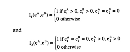
14 The basic setup is a one-shot setting. See Section 4.5 for a discussion of the effects of repetition.

The total benefit is then simply the sum of the benefit from initiative and the benefit from coordination:

R = R1 + Rc

It depends on the benefit parameters pA, pB and m and on the effort choices eA and eB.

Some of the benefits are realizations of random variables. To simplify the analysis, it is assumed that the benefits related to task 2, i.e. p2A, p2B, and m2 are fixed. Only the benefits related to task 1 are uncertain, as follows:

- the p1j are assumed to be distributed uniformly over [Lj, Hj] for j = A, B throughout
- various distributions for m, will be considered, but generally it will be assumed to be distributed uniformly over [LM, HM]

Unless stated otherwise, it will be assumed that Lj < p2j < Hj and similarly that LM < m2 < HM. All realizations are assumed to be independent of each other and across time.

4.2 Overview of the Analysis

This basic setup will be analyzed for a number of different assumptions about incentives and information. It functions much like a laboratory in which it is possible to conduct a variety of experiments. For incentives, two fundamental scenarios will be distinguished. In the team theory scenario, it is assumed that agents' incentives are aligned so that they will maximize the total benefit. In contrast, in the incentive scenario, it is assumed that agents maximize their individual benefits. The team theory scenario will be analyzed first and will provide a benchmark for comparison. 14

14 To the best of my knowledge there are no other papers that analyze several substantially different IT settings from both a team-theory and an incentive perspective.

Throughout, it will be assumed that the benefits from initiative are observed locally in the units, i.e. unit A observes pA and unit B observes pB. The benefits from coordination, m, are generally assumed to be observed by a central unit. Occasionally, it will also be discussed how the results would differ if the benefits from coordination were observed locally (e.g. if unit A observed and unit B observed m2). All observations occur before the units need to choose their effort levels and are realizations of random variables, as was described above. The availability and usage of IT determines how much of this information can be communicated between the units before efforts need to be chosen. Three settings will be distinguished, which coarsely reflect the evolution of IT, where IT is interpreted broadly to include both computation and communication.

  • No IT
    Without IT, communication is prohibitively slow and costly and hence the units must base their effort choices solely on their local observations of realizations and on the knowledge of the distributions of the variables. 15
  • Centralized IT
  • In the centralized IT setting, the local units can communicate the realizations pA and pB of the benefits from initiative to the center. The center thus has access to all information, including the realization m of the benefits from coordination. But the local units have limited computational power. Therefore, instead of being able to send all the information to the local units and letting them compute the optimal decision, the center must carry out the computation. The essence of such central computations is that they take a large number of inputs and reduce them to a few outputs. In order to avoid modeling difficulties, the output is assumed to be restricted to a single bit.16 This should not be seen as an asymmetry in the communication channel, but rather be compared to the information available to the respective sender: the local units send most (here: all) of their information, whereas the center carries out a computation and sends only the result.
15 This does not imply that communication is impossible; it is merely too slow and costly for the type of repeated observation and reaction considered here.
16 If the output were a real number, the center could potentially give highly sophisticated commands, which would be difficult to model. This problem is closely related to the information coding problem discussed in a separate paper (Wenger 1997a).
  • Networked IT
    Finally, with networked IT it is possible to share all observations. The units A and B can thus base their choice of efforts on a complete knowledge of all the benefits pA, pB, and m. The assumption here is that not only do high-speed networks make it possible to communicate all information, but there is also enough local computing power available to make use of it.

These assumptions about IT express capabilities only.17 Whether or not the units actually use these capabilities to truthfully report their observations is a separate issue. Truthtelling will be assumed for the team theory scenario but not for the incentive scenario.

4.3 Team Theory Scenario

4.3.1 Measures for Comparison

In order to have a unified way for comparing the results in the different settings and scenarios, it will be useful to introduce the following two measures:

  • Degree of Coordination
    Coordination will be said to occur when the units deviate from their locally optimal choice in order to obtain the coordination benefit.18 With perfect coordination the units only deviate when doing so is in fact optimal. There are three possible errors: deviation when it is not optimal (over-coordination); no deviation when it would be optimal (under-coordination); and wrong deviation (mis-coordination).19 The degree of coordination will therefore be the percentage of realizations of p1^, p1A and ml for which no coordination errors are made.
  • Degree of Initiative
    Initiative is the effort undertaken by the units. In order to separate its measurement from the measurement of coordination, the effort will be considered conditional on the choice of tasks. This is easiest by considering task 2 only, since for task 2 the benefit from initiative is fixed by assumption. The degree of initiative will therefore be the percentage of effort that is expended relative to the social optimum when task 2 is chosen.
17 The approach taken here is different from Malone and Wyner (1996). Their paper represents three organizational forms by reduced expressions that include both the cost and benefits from IT. The current paper, however, changes only the IT setting and treats the organizational form as endogenous.
18 This may appear to be an awkward definition, but its utility in measuring coordination will become apparent during the analysis.
19 For an example of mis-coordination consider the following: the locally optimal choices are task 2 for unit A and task 1 for unit 13; taking coordination into account, it would be optimal for both to choose task 2, yet they wind up both choosing task 1. They do coordinate, i.e. unit A deviates from the locally optimal task, but unit B should have been the one to deviate.

Both measures range between 0 and 100%. The rationale behind the particular choices of measures will become clearer as they are used below to compare various settings in the different scenarios.

4.3.2 Networked IT (Team Theory Scenario)

The Networked IT setting is the easiest to analyze since here all information can be communicated. With costless communication, it is always optimal in a team theory setting to actually communicate all the information (Marschak and Radner 1972). The team members can then each solve the overall optimization problem and locally make their choices according to this socially optimal solution. The Networked IT setting in the team theory scenario also provides a natural base for comparison. All other situations involve some type of constraint on the available information, the incentives, or both.

The decision rule for the Networked IT setting can be derived as follows. Given the assumptions, it is never optimal for a local unit (A or B) to split its effort between the two tasks. Suppose splitting were optimal. This would result in

Rc = m • I(eA eB) = (m1, m2)' • (0,0) = 0

But with no benefit from coordination, the benefit from initiative can be maximized freely (there can be no loss of coordination benefit). Since the benefit from initiative is linear by assumption, it is optimal for each unit to allocate all effort to the task with the higher benefit. Hence, splitting could not have been optimal.

With splitting ruled out, the decision rule consists of comparing the total benefit from four different possible optimizations (depending on which tasks are chosen, as indicated in the first two columns):

A B Optimization
1
1
2
2
1
2
1
2
max p1A . e1A + p1B . e1B + m1 - 1/2(e1A - E0)2 - 1/2(e1B - E0)2
max p1A . e1A + p2B . e2B - 1/2(e1A - E0)2 - 1/2(e2B - E0)2
max p2A . e2A + p1B . e1B - 1/2(e2A - E0)2 - 1/2(e1B - E0)2
max p2A . e2A + p2B . e2B + m2 - 1/2(e2A - E0)2 - 1/2(e2B - E0)2

As can easily be seen, all four of these optimizations are completely separable into an optimization for unit A and one for unit B. Each of the smaller problems is of the form

max p1j • eej - 1/2 (e1j-E0)2   for i = 1,2 and j = A, B

with the solution

e1j* = p1j + E0 for i = 1,2 and j = A, B

The socially optimal effort choice for task 2, e2j*, will later be used to compute the degree of initiative. It is now straightforward to determine the optimized values and compare them in order to determine the optimal choice of tasks.

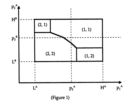
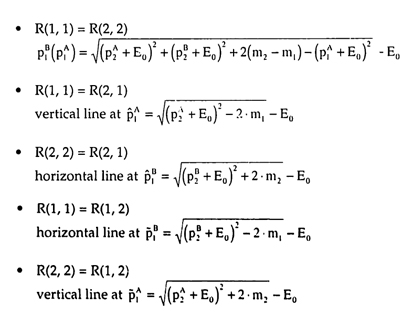
Given the assumptions about the structure of the uncertainty, there is a convenient way of graphing the resulting decision rule. For a given realization of m, the optimal choice of tasks can be graphed as a phase diagram in (p1A, p1B) space, since p2A, p2B, and m2 are fixed by assumption. The shape of the phase diagram is derived in Appendix A and shown in Figure 1.

The notation (A, B) indicates the tasks to which the units should optimally allocate their effort for each region of the phase diagram. It is important to note, that while the shape of the diagram is always the same, the exact size of the regions depends on the benefit from coordination. With m2 fixed by assumption, the size depends on the realization of m1 As is shown in Appendix Al, for m1 = m2, the curve separating the (1,1) and (2,2) regions passes right through the point (p2A, p2B). For m1 > m2, the curve passes below the point and for m1 < m2, the curve passes above it.

Using this phase diagram, the decision rule can be stated in the following way that facilitates the further analysis and clarifies its implications:

Networked IT Decision Rule
  1. Communicate all information. Then determine to which task to allocate effort by drawing the phase diagram for the realization of m{ and seeing in which region the point (p1A, p1B) falls.
  2. Choose the effort level for the correct task according to e1j* = p1j + E0 .

In this formulation, part 1 of the decision rule takes care of coordination, i.e. the choice of task. From the derivation it follows that 100% coordination is achieved. Part 2 of the decision rule determines initiative, i.e. the degree of effort. Again, it follows from the derivation that 100% initiative is achieved.

As will be seen shortly, in the team theory scenario, changes in the IT setting affect only part 1 of this decision rule and hence the degree of coordination. Part 2 remains the same and hence there is always 100% initiative. This separability is not really a result, since it was built in by assuming that the coordination benefit is independent of the level of effort. The reason for making this assumption is to clarify the source of the tradeoff between initiative and coordination: In the incentive scenario, separability breaks down, and a tradeoff between initiative and coordination exists.

Another implication of the decision rule for Networked IT is noteworthy. The central unit's only role is to communicate its observation of the benefits from coordination. The central unit is not required for decision making, since the required decision-making can take place in a decentralized fashion in the local units. Therefore if unit A were to observe ml and unit B were to "observe" m2 (it is assumed to be fixed), or the other way round, there would be no role at all for a central unit.

4.3.3 Centralized IT (Team Theory Scenario)

With Centralized IT, the central unit can obtain all information: it observes the realization m of the benefits from coordination and the local units A and B can communicate their respective benefits from initiative, pA and pB, to the center. The central unit can now draw the phase diagram and determine the optimal choice of tasks. It can then use the two single bits to communicate the task choice back to the units, e.g. bitj = 0 means "choose task 1" and bitj = 1 means "choose task 2" (for j = A, B). This is summarized in the following decision rule:

Centralized IT Decision Rule
  1. Communicate local observation to the center, which will send back the correct task.
  2. Choose the effort level for the correct task according to e1j* = p1j + E0.

In the team theory scenario, Centralized IT can thus achieve exactly the same outcome as Networked IT, i.e. 100% coordination and 100% initiative. Now, however, the central unit plays a crucial role, since it actually chooses the correct tasks. Once each local unit has received its central command, it can choose the optimal effort level, since this only requires it to know the benefit from initiative which it has observed locally. Again, the analysis would not change much if the benefits from coordination were also observed locally.

4.3.4 No IT (Team Theory Scenario)

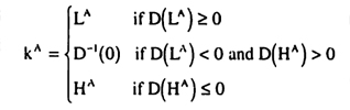
Without IT, the units must base their choice of tasks solely on their local observation of the benefits from initiative and their knowledge of the distribution of the benefits from coordination. In Appendix A2 it is shown that the following simple decision rule is optimal for this setting:

No IT Decision Rule
  1. If p1j is above the cutoff k1, choose task 1. If it is below the cutoff, choose task 2.
  2. Choose the effort level for the correct task according to e1j* = p1j + E0.

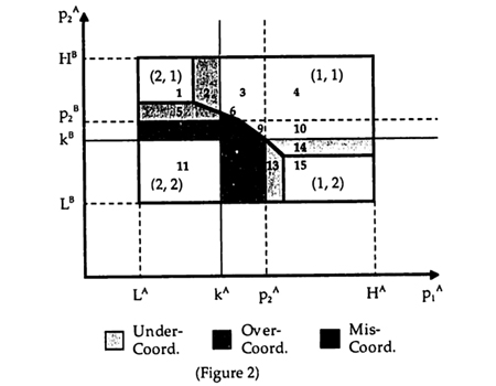
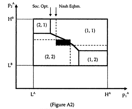
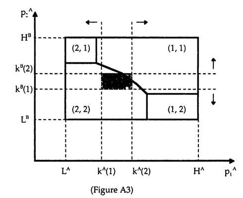
Without IT, it will—in general—no longer be possible to achieve perfect coordination. Consider the following phase diagram which was drawn for a particular (albeit unobserved) realization of m1

The thick lines in Figure 2 mark the areas for the optimal task choices, which are indicated in the four comers. The solid lines at kA and k" determine the four quadrants of actual task choices, whereas the dotted lines at p2A and p2B determine the four quadrants of locally optimal choices. The following table summarizes the choices for each area:

Area Optimal Local Actual Coordination
1 (2,1) (2,1) (2,1) none required
2 (ID (2,1) (2,1) under
3 (l,D (2,1) (1,1) optimal
4 (l, l) (1,1) (1,D none required
5 (2,2) (2,1) (2,1) under
6 (2,2) (2,1) (1,1) mis
7 (2,2) (2,2) (2,1) over
8 (2,2) (2,2) (1,1) over
9 (1,1) (2,2) (1,1) optimal
10 (1,1) (1,2) (1,1) optimal
11 (2,2) (2,2) (2,2) none required
12 (2,2) (2,2) (1,2) over
13 (2,2) (1,2) (1,2) under
14 (1,1) (1,2) (1,2) under
15 (1,2) (1,2) (1,2) none required

As Figure 2 and the summary table show, there are areas in which coordination errors are made. In areas 2,5,13, and 14 coordination would be required but does not take place (under-coordination). In areas 7,8, and 12 coordination is not required but does take place (over-coordination). Finally, in area 6 coordination is required, but the wrong coordination occurs (mis-coordination). Hence the degree of coordination is strictly less than 100%.

The degree of coordination is lowest for "moderate" distributions of the benefits from coordination, i.e. when coordination matters but is not overwhelming. The closer the distribution is to one of two extreme cases, the higher the degree of coordination. The first extreme case occurs when there are no benefits from coordination (m1, = m2 = 0 always). The second extreme case occurs when the benefits from coordination are so overwhelming that a unique choice of tasks (e.g. both units always choosing task 1) is optimal. In both extreme cases 100% coordination can be achieved even without IT.

Without IT, there will be a significant difference if the benefits from coordination are observed by the local units. In particular, if unit A were to observe it would condition its cutoff on the observation, i.e. kA(m1). It is easily seen that the cutoff would have to be lower for higher realizations of m1.

4.3.5 Summary of Team Theory Scenario

The analysis of the team theory scenario thus provides a number of important insights.

  • The degree of initiative is 100% for all IT settings.
  • In both the Networked IT and the Centralized IT setting, 100% coordination can be achieved for any distribution of the benefits from coordination.
  • In the No IT setting, coordination degrades, with the degree of coordination being worst, when both initiative and coordination matter.

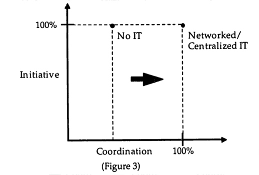
These insights can be summarized in the following diagram (Figure 3), which will later be used for comparisons to the incentive scenario.

Figure 3 assumes distributions of the parameters for which both the benefits from initiative and the benefits from coordination matter. The dots mark the maximum coordination that can be achieved for each of the IT settings. The dotted lines indicate that in each IT setting it is also possible to have less coordination and/or less initiative, if a non-optimal decision rule were used. For instance, in the No IT setting, if the cutoff in the decision rule is too low or too high there will be less coordination than can be achieved with the optimal cutoff.

In other words, the dotted line is the initiative - coordination frontier for an IT setting. More IT shifts the frontier to the right as indicated by the arrow. Given the definitions of the measures, more initiative and more coordination are desirable. Therefore given the rectangular shape of the frontiers, the uniquely optimal point is as indicated in the top right comer.

4.4 Incentive Scenario

4.4.1 Additional Assumptions

The team theory scenario is built on the premise that all agents will optimize the overall benefit rather than their individual benefits. In most organizational settings this is rather unrealistic. Introducing incentive issues affects the analysis in two major ways. First, agents will choose effort to maximize their own benefit given their incentive scheme. Second, agents will not necessarily truthfully reveal the information available to them but must be given incentives to do so.

The incentives will be based on two measures of the benefit, one for unit A and one for unit B, as follows:

RA = R1A + 0.5 - Rc = pA • eA + 0.5 • m - I(eA, eB)
RB = R1B + 0.5 • Rc = pB • eB + 0.5 • m - I(eA, eB)

It can easily be seen that the two measures sum to the total benefit. The measures reflect the idea that the benefit from coordination cannot be attributed to either unit and is therefore split between them. This could be the result of an allocation rule by the center or the outcome of a bargaining process between the two units. 20

The analysis will be restricted to incentive schemes that are linear in these two measures. The "wages" for the two units thus take the following form:

wA = α0 + αA . RA + αB . RB
wB = β0 + βA . RA + βB . RB

The weights on the two measures will often be referred to as the "commission rates," They should be interpreted as a reduced form representation of a large number of incentive instruments, which include explicit commissions, but also include ownership, subjective performance measures and others.

20 If there were N units then this model would represent a coordination opportunity between any two of them. Alternatively, one could explore the effects of a situation where the coordination benefit is spread across many units.

Focusing on linear schemes is less restrictive than it may at first appear. The units can observe the realizations of at least some of the benefit parameters before making their choices. Therefore they can condition their level of effort on their observations. In such a case, non-linear schemes can result in large distortions, and it has been shown that linear schemes may be optimal (Holmstrom and Milgrom 1987).

The measures also intentionally do not include the cost of effort. If the cost were completely measurable, there would be no incentive problem. By setting the commissions to αA = αB = βA = βB =0.5, each unit would face exactly the same optimization problem as in the team theory scenario (scaled by a constant factor of 0.5, but that of course does not affect the choices). The assumption that cost cannot be measured is readily justifiable when the units are individuals since effort costs are subjective and therefore impossible to measure directly. In the case of businesses allocating resources, the assumption may appear less justified since one might argue that accounting cost could be used. This would, however, not be appropriate for two reasons. First, the units are likely to have many activities (aside from the ones modeled), and hence their accounting cost is subject to various manipulations, such as the allocation of overhead. Second, the relevant cost concept are opportunity costs, which may diverge widely from the recorded accounting cost even without any manipulation. Third, the cost may reflect additional personal costs or benefits to the managers of the businesses, which are difficult to measure.

4.4.2 Networked IT (Incentive Scenario)

To analyze the Networked IT setting, it will first be assumed that both units truthfully report their information. Note that the revelation principle cannot be applied here since the contracts have been restricted to linear schemes. The remaining incentive problem is then the choice of effort. Consider Unit A's optimization problem, treating Unit B's effort choices as given

max wA - c(eA) =
= max α0 + αA • pA' • eA + (αA + αB) - 0.5 • m'. I(eA, eB) - 0.5(e1A + e2A - E0)2

By the same argument as in the team theory scenario, it is never optimal for Unit A (and hence also for Unit B) to split its effort between the two tasks. Therefore Unit A's optimizations can be reduced to two smaller problems of the form

max αA . piA . eiA- 1/2 (eiA - E0)2 for i=1,2

with the solutions

eiA* = αA . piA + E0 for i = 1,2

The problems and solutions are analogous for unit B.

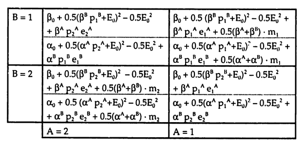
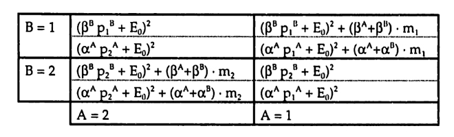
Given these solutions and the fact that neither unit will split its effort between the two tasks, it is straightforward to represent the game played between the two units in normal form (the relevant simplifications are shown in Appendix A3.1). 21

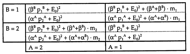
21 The somewhat unusual layout of the normal form was chosen to reflect the orientation of the phase diagram from the team theory scenario.

By inspecting the normal form, it is possible to discern the effects of changes in the various commission rates (see Appendix A3.2 for a more formal analysis, as well as Section 4.5 for a discussion of the effects of repetition):

  • αA and βB
    These commission rates affect all four payoffs for units A and B respectively. But their relative effect is stronger for payoff terms without coordination benefit (i.e. A = 1 / B = 2 and A = 2 / B = 1). Hence decreasing these rates makes the outcomes with coordination benefit more likely. This effect can be understood best by examining the special case of αA = βB = 0.
  • αB and βA
    These commission rates affect only the payoff terms with coordination benefit (i.e. A = 1 / B = 1 and A - 2 / B = 2). Hence increasing these rates makes the outcomes with coordination benefits more likely. This effect can be understood best by starting with αA = βB = 0.5 and αB = βA = - 0.5 and then increasing both αB = βA to 0 or even to positive 0.5.

The commission rates thus have different effects and can be used to guide the game played between the two units.

Two special cases, the individual entrepreneurs and the bureaucracy, will provide additional intuition.

  • αA = βB = 1 and αB = βA = 0
  • These commission rates correspond to the case of individual entrepreneurs who own their respective businesses, They are residual claimants and thus obtain their full benefit, including a 50:50 split of the benefits from coordination as the result of bargaining between them. The first insight is that in this case the conditions for the choice of effort are the same as in the team theory scenario
    eiA* = αA • piA + E0 = piA + E0
    eiB* = βB • piB + E0 = piB + E0
    Hence the degree of effort is the same, i.e. 100%. The second key insight is that the degree of coordination is lower than in the team theory scenario. The intuition is that coordination requires deviations from the locally optimal choice. Since the entrepreneurs obtain the full benefits from initiative but only half the benefits from coordination, they will deviate less frequently from the locally optimal choice than would be necessary for 100% coordination.22
  • αA = αB βA = βB = 0
    These commission rates correspond to the case of bureaucracy. The units have no ownership and do not receive any explicit incentive pay. The combination of the various incentive instruments results in wages that are completely flat, i.e. the individual benefits are fixed. By inspection of the optimization problems from above, it follows immediately that the effort level will drop to E0. The degree of effort is thus less than 100% as long as p2j > 0 for j = A, B
    E0 / (p2j + E0) < 1 if p2j > 0
    Bureaucracy, however, can achieve 100% coordination. The payoffs in the normal form are E02 everywhere and the units are thus indifferent between the choices of tasks.

The two special cases thus fit the intuition that was developed earlier for the tradeoff between initiative and coordination.

The question immediately arises whether it is possible to achieve both 100% initiative and 100% coordination as in the team theory scenario. One might consider giving both units the full benefit by setting αA = αB = 1 and similarly βA = βB = 1. The problem with this solution is that it uses up twice the benefit that is available. In other words, it does not meet the budget constraint of

WA + WB ≤ R

It is only possible to give the full marginal benefit to one of the two units, in which case the other unit will exert minimal effort E0. Any solution that meets the budget constraint cannot achieve both 100% initiative and 100% coordination. It is important to note that this is a result of using continuous schemes. Suppose that all the realizations of the parameters were known in advance.23 Then it would be possible to calculate the maximal benefit and to use a discontinuous incentive scheme which gives nothing to the units unless they achieve the maximal benefit. Such a scheme is known as "budget breaking" and can achieve 100% initiative (Holmstrom 1982). However, as was pointed out above, such discontinuous schemes tend to not work well when the realizations are observed before the actions are taken. The case study section and the section on managerial implications will relate this to the increased use of "stretch targets" and "mission statements" in hybrid organizations.

The budget constraint in combination with the linear incentives thus imposes a tradeoff between initiative and coordination. Characterizing this tradeoff turns out to be rather difficult. If one considers the (p1A, p1B) space, then changes in the commission rates have two effects. First, the rates affect the game played between the two units and thus determine which set of equilibria is possible for given realizations. Second, they also shift the boundaries of the phase diagram for the socially optimal choices, since the commission rates affect the level of effort, This effect is like chasing a moving target: changes to the commission rates influence both how the units will play and how they should play. Because of this complexity, the actual analysis is relegated to Appendix A3 2 and only the results are shown here.

22 This is shown formally in Appendix A3.2.
23 The following argument also works under uncertainty, but onJy to the extent that the agents do not observe the realizations before they take their actions.

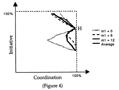
As in the team theory scenario, the approach for the analysis is to first take realizations of the benefits from coordination as given. The following figure shows the conditional initiative - coordination frontiers for selected realizations of m1 as colored lines (m2 = 6). Each frontier is the result of varying the commission rates. First αA and βB are chosen between 0 and 1, which fixes the degree of initiative. Then αB and βA are determined to maximize the degree of coordination. The actual frontier is found as an average across all realizations and is indicated as a solid black line.

Figure 4 provides some important insights into the organizational implications of Networked IT.

  • First, for every realization it is possible to achieve close to 100% coordination for a level of initiative that is significantly above the bureaucratic minimum. This is a crucial observation since it helps explain the idea of hybrid organizations. The point where all curves reach almost 100% coordination will be referred to as the "hybrid point" (labeled H in Figure 4). The hybrid point is marked by balanced incentives: each unit's "wage" depends both on its own performance and on the performance of the other unit.

  • Second, one can see clearly that as the degree of initiative rises above the hybrid point and approaches 100%, the degree of coordination degrades. The degradation is strongest when the coordination benefit is the same for both tasks (i.e. m1 = m2 = 6), as indicated by the green line. Interestingly, ordination also degrades for levels of initiative below the hybrid point. The error here is over-coordination, i.e. the units deviate too frequently from the local optimum.

  • Third, it is no longer easily possible to determine the optimal point, as was the case in the team theory scenario. Most points below the hybrid point are clearly dominated since they involve both less coordination and less initiative. Above the hybrid point, however, there is an important tradeoff: more initiative implies less coordination. Interestingly, the hybrid point while not necessarily optimal, will be quite good for a large range of situations whereas 100% initiative does quite poorly for some realizations. This stability further increases the appeal of hybrid organizations. While they may not be optimal for any particular situation, they may be close to optimal for a large number of situations and are thus quite robust.

These insights will be explored in more detail below during the discussions of historical and case study evidence and of managerial implications.

The analysis up to this point has assumed that both units will truthfully report their observations. In Appendix A3.3 it is shown that this will not necessarily be the case. It turns out that emphasizing initiative increases the units' incentives to misrepresent their observations. The balanced incentives found in hybrid organizations thus have the added appeal that they encourage the truthful reporting of information. This factor will be even stronger when the units also observe the coordination benefits, i.e. when unit A reports the realization of m1. This suggests an additional insight for the organizational implications of Networked IT: there may be a role for a center in enforcing truthful reporting. Such enforcement may in fact be supported by Networked IT itself, for instance in the form of more detailed audit trails.

4.4.3 Centralized IT (Incentive Scenario)

As in the Networked IT setting, it will at first be assumed that the units truthfully report their observations.24 It is thus still possible for the central unit to determine the optimal choice of tasks. But the local units will no longer necessarily carry out the central unit's command. Instead, the units will again play a game. This game will now be analyzed. The analysis turns out to be surprisingly similar to the analysis of the No IT setting in the team theory scenario, as presented in Appendix A2.

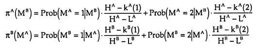
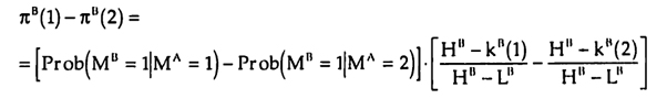
Let лB(MA) denote the probability that unit B will choose task 1, given that unit A has received the message MA = 1,2 from the central unit (note that the actual message is a single bit and hence either 0 or 1). Unit A will choose task 1, when its expecied benefit E[A1] is larger than the expected benefit from task 2. In Appendix A4.1 it is shown that the choices of effort for unit A are determined by

eiA* = αA . piA + E0

and that the difference in expected benefits is

D(p1A, MA) := E[A1] - E[A2] = (αA p1A + E0)2 - (αA p2A + E0)2 +
+(αA + αB) . {лB (MA) E[m1 | MA] - (1-лB(MA)) . m2}

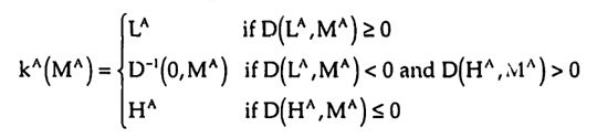
The difference between expected benefits is continuous and strictly increasing in p1A. Hence there exists a cutoff kA(MA) such that for p1A ≥ kA(MA) the difference in expected benefits is non-negative, i.e. D(p1A, MA) ≥ 0, and hence unit A will choose task 1. The logic is analogous for unit B.

24 As before, it is not possible to apply the revelation principle.

Several insights can be gained by inspecting the determination of the cutoffs. As in the Networked IT setting, the commission rates αA and βB affect the importance of both the benefits from initiative and the benefits from coordination. The commission rates αB and βA on the other hand affect only the importance of the benefits from coordination. It follows immediately that more coordination can be achieved when the incentives are more balanced. The two special cases are also very similar to the Networked IT setting.

  • αA = βB = 1 and αB = βA = 0
    For individual entrepreneurs it is again true that the degree of initiative is 100%. This follows immediately from the equations for optimal effort. The degree of coordination, however, will generally be less than 100%. For any realization of p1j > kj(2) unit j = A, B will choose task 1 despite the central unit's message. Again the intuition is that since the entrepreneurs obtain the full benefits from initiative but only half the benefits from coordination, the units will deviate less frequently from the locally optimal choice than would be necessary for 100% coordination.

  • αA = αB = βA = βB = 0
    In the case of bureaucracy it again follows immediately that the effort level will drop to E0 and hence that the degree of effort is less than 100%. Bureaucracy, however, can achieve 100% coordination. The units are now indifferent between the two tasks and hence will follow the central unit's command.

The analysis of the intermediate cases requires a characterization of the equilibrium, which is cumbersome and therefore relegated to Appendix A4.2.

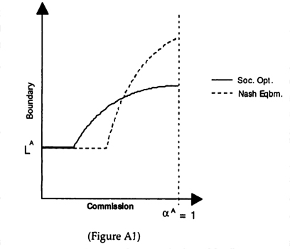
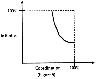
Based on the characterization of the equilibrium from Appendix A4.2 it is possible to give a rough sketch of the initiative - coordination frontier as shown in Figure 5. For high values of αA and βB, initiative is high, but the cutoffs kj(l) and kj(2) are close together resulting in under-coordination. As the incentives become more balanced, the cutoffs move further apart. While this improves coordination, it is not possible to achieve 100% coordination. The achievable degree of coordination depends on the distribution of m,. The stronger the variation in m1 the less coordination can be achieved since the cutoffs are fixed. As the commissions are lowered further, coordination continues to improve as initiative declines. As was shown in Appendix A4.2, the area in which perfect coordination can be achieved grows at an increasing rate, thus explaining the curvature of the frontier. Finally, by setting commissions to 0, it is possible to achieve 100% coordination with minimal initiative.

Figure 5 provides several important insights into the organizational implications of Centralized IT.

  • First, the only way to achieve 100% coordination is by reducing initiative to the minimal level by setting all commissions to zero. This extreme point has previously been interpreted as a bureaucracy with flat wages and no ownership. Centralized IT thus favors a bureaucratic organization when coordination is important.

  • Second, the only way to achieve 100% initiative is with substantially reduced coordination. This extreme point has previously been interpreted as individual entrepreneurs.

  • Third, there is a strong tradeoff between initiative and coordination, i.e. as incentives are increased initiative improves, but coordination degrades. The curvature of the tradeoff suggests that the optimal point is likely to be one of the two extremes of either bureaucracy or individual entrepreneurs.

These insights will be explored in more detail below during the discussions of historical and case study evidence and of managerial implications.

Again, the assumption that the units will truthfully report their observations should be revisited. For the bureaucratic extreme this will obviously be true since the units are indifferent between all the outcomes. However, when initiative is emphasized and especially in the individual entrepreneurs case, the units have an incentive to misrepresent their information. For instance, by over-reporting the realization of p1A, unit A may get the central unit to send out Mj = 1 to both units when for the true realization the messages would have been Mj = 2. Unit A may benefit from this change in messages since it retains 100% of the benefit from its effort, but only 50% of the benefit from coordination. The problem will be especially pronounced when unit A is also in charge of reporting the realization of m1. In addition to processing the information and issuing the messages, the center may thus have to ensure truthful reporting. Note that all of these activities are costly for the center and hence for the individual entrepreneurs case, the central unit will likely have to charge a flat fee, i.e. α0, β0 < 0.

4.4.4 No IT (Incentive Scenario)

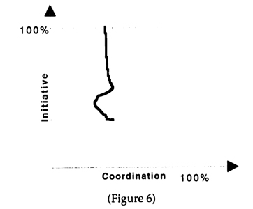
Without IT there is no reporting and hence no assumption about truthfulness needs to be mode. The units play a game based solely on their own observations. In the team theory scenario, the optimal decision rule consisted of a cutoff. The equilibrium of the game played by the units in the incentive scenario will involve a similar cutoff. This follows directly from the analysis of the Centralized IT setting given above. The strategies there were conditioned on a message from the central unit, which resulted in two different cutoffs. Therefore, without a message from the central unit there will be only a single cutoff. The analysis, which is carried out in Appendix A5, thus consists of comparing the socially optimal cutoff with the equilibrium cutoff. The resulting initiative -coordination tradeoff is depicted in Figure 6.

Figure 6 provides several important insights into the organizational implications of No IT.

  • First, without IT it is impossible to achieve 100% coordination. The highest possible coordination is the same as in the team theory scenario, as indicated by the dashed vertical line. Interestingly, this can be achieved at a degree of initiative that is above the bureaucratic minimum.

  • Second, as the degree of initiative approaches 100%, the degree of coordination declines, but only moderately. Even for 100% initiative the degree of coordination is close to the team theory scenario. Hence, while there is a tradeoff between initiative and coordination, it appears likely that the optimal point is at 100% initiative.

These insights will be explored in more detail below during the discussions of historical and case study evidence and of managerial implications.

4.4.5 Summary of Incentive Scenario

The analysis of the incentive scenario thus provides a number of important insights.

  • As the degree of initiative rises towards 100% there is a tradeoff with coordination in all IT settings.

  • IT expands the tradeoff frontier. With Centralized IT, it is possible to achieve both more coordination and more initiative than without IT, and Networked IT expands the frontier even further.

  • The different IT settings favor different organizational forms. Without IT, the individual entrepreneur form is favored. Centralized IT favors a bureaucratic form of organization. Finally, Networked IT favors hybrid organizations.

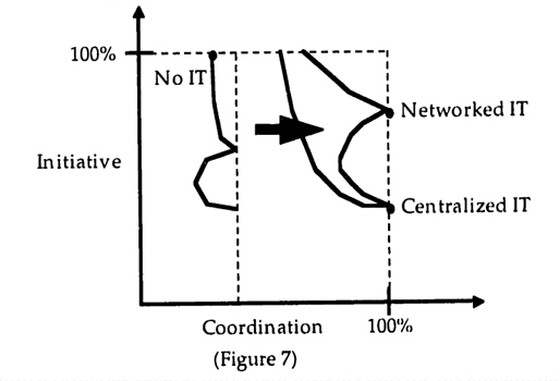
These insights can be summarized by combining the various tradeoff frontiers into a single diagram (Figure 7).

Figure 7 shows how the increased availability of IT expands the tradeoff frontier as indicated by the arrow. The dots indicate the points on the frontier that are favored by the different IT settings. The dashed lines indicate the team theory scenario as depicted in Figure 3. Given the assumptions of the model, the resulting historical evolution of organizations thus proceeds in three stages:

Stage Use of IT Preferred Form of Organization
1 No IT Individual Entrepreneurs
2 Centralized IT Bureaucracy
3 Networked IT Hybrid Organization

This is clearly a highly reduced summary of the analysis. For instance, for certain settings the benefits from initiative may be so important that individual entrepreneurs are the preferred form of organization no matter what the degree of IT use. Nevertheless, the particular pattern of individual entrepreneurs to bureaucracy to hybrid organization should apply to a large number of settings. It has also been identified in work by Malone and Wyner (1996). Sections 5 and 6 present historical and case evidence to support the relevance of this pattern.

4.5 Repetition

The modeling has thus far ignored the issue of repetition. In many organizational settings of interest, the allocation of effort or resources that requires coordination will occur repeatedly. This raises the question how repetition will affect the results of the analysis. For the team theory scenario the answer is simple: repetition has no effect. First, there are no incentive considerations that could be affected. Second, by assumption, the random variables are uniformly distributed and independent across repetitions so that no additional information becomes available.

In the incentive scenario, repetition plays a more important role since it affect the strategies available to the units. Consider the case of networked IT. Suppose further that eventually it will always be revealed whether or not a unit truthfully reported the information that it observed. Then it might be possible to find an equilibrium that achieves both 100% initiative and 100% coordination. The threat of a "grim" strategy of always playing the local optimum, or even intentionally choosing the task that minimizes the other unit's payoff, may suffice to get both units to optimally coordinate and exert the optimal effort.

A detailed analysis of the repeated game is beyond the scope of the current paper but is an important issue for future work.25 It would, however, be surprising if the kind of equilibrium existed that overcomes the coordination-initiative trade-off. Most organizational settings are quite dynamic, thus limiting the frequency of repetition. Career and financial concerns often contribute to an emphasis on short-term results, thus effectively giving individuals and businesses high discount rates. In combination these factors significantly reduce the effectiveness of strategies that rely on future punishment to prevent current deviations. The main expected result from an analysis is thus that repetition will make it possible to sustain higher levels of both coordination and initiative than in the one-shot setting without eliminating the fundamental trade-off.

25 For an interesting related analysis see Baker, Gibbons, and Murphy (1995).

5. Historical Evidence

5.1 Purpose

IT includes technology for both processing and communicating information. When interpreted broadly, IT encompasses such "primitive" technologies as pencil and paper. IT thus has a long history, and its influence should be reflected in historic developments in the design of organizations. This section presents several examples of historic changes and argues that they show a pattern which is consistent with the model analyzed above. While these examples by no means constitute a test of the model, they show how the model provides a useful structure for examining evidence and in turn may strengthen one's belief in its validity.

5.2 Military Organization

Armies have for a long-time been held to belong to the precursors of other large-scale organizations. From early management theorists, such as Fayol (1949), to recent management books (e.g. Dunnigan and Masterson 1997), authors have looked at military organization for insights. Conversely, given its nature (and frequently its funding) the military has often led the adoption of new technologies and thus provides fertile ground for examining their impact.

Consider first the difference between guerrilla troops and traditional armies, as seen recently in the Russian invasion of Afghanistan. Guerrillas generally rely on relatively primitive communication (e.g. handheld radios). They also tend to have little or no heavy equipment, such as tanks or airplanes, that would require significant coordination in order to be effective (e.g. logistics for parts and fuel). Instead, much of their effectiveness depends on the ability to rapidly seize an opportunity for attack and quickly disappear. The guerrillas represent the No IT model of warfare. Small units act more or less on their own and get the full benefit (e.g. in the form of reputation) or downside (e.g. nobody coming to the rescue) of their actions. Traditional armies, on the other hand, represent the Centralized IT model of warfare. They have decision-making centers at the top of a hierarchy, which accumulate information, make decisions, and then pass commands back down. The lower levels carry out the commands and usually have little to no authority to deviate from the commands based on the local situation. Much of the effectiveness of traditional armies depends on the deployment of large troop contingents and the intensive use of heavy equipment, both of which require substantial degrees of coordination.

There is, however, a new model of warfare emerging, which roughly corresponds to the Networked IT setting. While there is still central gathering of information and decision-making, much more information is made available to all levels. This permits troops on the ground to make decisions based on both the local and the overall situation. Operation Desert Storm was a first visible example of this approach (Blackwell 1991; Clancy and Franks Jr. Ret. 1997). For instance, the US forces were using a joint logistics information system, which permitted troops to find out instantly where supplies were (including those in transit). Another system provided real-time location tracking of all deployed troops and equipment, such as tanks and artillery, enabling lower levels to make deployment decisions. This system made it possible to integrate troops from many different nations and to advance quite rapidly.

5.3 Automobile Industry

To this day, automobile production is a significant factor in the economies of several of the leading industrial nations. Many other manufacturing industries have followed patterns observed first in the automotive industry. Given the large fortunes at stake, the automotive industry has also frequently been an early adopter of new technologies. The organization of automobile production is therefore a topic of great interest.26

The early automobile pioneers were often inventors or engineers who set up a small shop to manufacture cars almost completely manually. This craft mode of production heavily emphasized individual skill and initiative. It occurred in essentially a No IT setting, simply because at the time the available means of communication was quite primitive. A major change occurred with the introduction of the assembly line and the shift towards mass production as initiated by Ford. Following the methods of Taylor, work was broken down into tiny steps, and coordination rather than initiative became crucial. This mode of production coincided with improvements in IT, such as the widespread availability of telegraphs and centrex telephones (i.e. within one plant), which resulted in a Centralized IT setting. Information gathering and decision-making was essentially highly centralized. Commands were then issued from the center. In order to be able to issue commands backward in the supply chain, one of two models was generally chosen; Automobile manufacturers were either vertically integrated into parts production or held large inventories of parts.

26 For instance, the study of automobile manufacturing in Womack, Jones, and Roos (1990) is generally credited with having contributed significantly to the diffusion of so-called lean manufacturing techniques to other industries.

The Japanese pioneered a new mode of production, which has become known as lean or modern manufacturing (Womack et al. 1990). This new mode was originally born out of necessity. The Japanese needed to catch up with other nations, which required rapid innovation and thus, given their initially small domestic market, short production runs. The frequent changes ruled out both vertical integration and large inventories as solutions. Instead, the Japanese relied from the beginning on suppliers to create larger components rather than individual parts, and to deliver these just-in-time QIT). An advantage of starting from scratch was that they could co-locate the suppliers and the assemblers. This permitted an intense exchange of information, as in a Networked IT setting, even using relatively primitive forms of IT such as manually transmitted cards.

Today, lean manufacturing is widely diffused and practiced by auto¬mobile producers around the world. It is also tied intimately to intense information sharing, which is generally accomplished through sophisticated computer networks.27 The automotive industry, for instance, pioneered the use of Electronic Data Interchange (EDI). EDI requires that all participants in an industry agree on a standard method of encoding various business transactions into electronic messages. These messages can then be exchanged and processed automatically. In the automotive industry there are many EDI messages that notify suppliers about the planned production so that the suppliers can coordinate their own production schedules in advance.28

27 For an empirical analysis of the relation between the supplier practices associated with lean manufacturing and the degree of information sharing, see Helper and Sako (1995).
28 See the relevant ANSI standards.

6. CASE STUDY EVIDENCE

6.1 Purpose

Case study evidence is a natural complement to historical evidence. Instead of broad trends, a case study focuses on a single firm to illustrate in great detail the richness of organizational design problems. In particular, a case study provides a vehicle for examining a multitude of different design instruments, which in the model were reduced to two commission rates. The effects of other simplifications, such as considering linear schemes only and analyzing games as one-shot, can also be considered.

6.2 Background

The case study draws on evidence that was collected over the course of three years of consulting work for Siemens Nixdorf Informationssysteme (SNI), which is a wholly owned subsidiary of Siemens AG.29 For the 1996 fiscal year, SNI had worldwide revenues of DM 13.6 billion, of which about 60% came from Germany, 30% from the rest of Europe and 10% from the rest of the world. SNI was the result of a merger between the ailing Nixdorf company and the IT unit of Siemens AG in 1990. After the merger, SNI accumulated substantial losses of almost DM 2 billion. In 1994, Gerhard Schulmeyer, an alumnus of MITs Sloan Fellows program and former executive at ABB and Motorola, became the new CEO of SNI and initiated a radical change program aimed at transforming SNI into a hybrid organization that would combine high degrees of both coordination and initiative.

6.3 The Need for a Hybrid Organization

SNI belongs to the shrinking group of surviving "first generation" computer companies. These companies were started in the mainframe era of computing and supply a very broad product-line. On the hardware side, the product line ranges from PCs and Point-of-Sales terminals via mid-range computers to large mainframes and massively parallel computers and also includes printers, other peripherals, and networking equipment. On the software side, the product line ranges from low-level systems software to end-user applications. While some of the products are "pass-throughs," many are produced in-house. In addition to the products, these companies also supply a wide variety of services, including outsourcing, consulting, and systems integration.

29 I am deeply grateful lo Gerhard Schulmeyer, the CEO of SNI, for having provided me with outstanding access to the entire organization and for having taken time on numerous occasions to dicuss the concept of hybrid organizations with me.

The IT marketplace requires extensive initiative. The competition is fierce and the technology is changing rapidly. The changes in technology are frequently not incremental but rather offer completely new solutions. Much of this innovation is driven by new and at least initially more focused companies such as Microsoft and more recently Netscape. Yet there is also a tremendous need for coordination. As more computers are connected to networks, these computers need to be able to work together with other computers. This integration requires compatibility of the systems on both the hardware and software levels. While standards exist that are aimed at ensuring compatibility, in reality systems from a single vendor tend to work together much better than a standards-based integration of systems from multiple vendors.

For instance, IBM is currently the most successful of the "first generation" survivors. The former CEO, Akers, had embarked on a strategy of attempting to break up IBM into completely separate pieces, most likely with the goal of selling some of them. The current CEO, Gerstner, decided instead to keep the company mostly intact (the printer division was spun-off, but IBM has since started producing its own printers again). Similarly, Microsoft, has gradually enlarged its product range to include all types of software (and more recently entertainment). Microsoft has been able to do so based on its widely distributed operating system. Even though Microsoft has published the access standards for much of its software, third party software tends to integrate less well than its own products.30 Even Netscape, which is basing much of its software on completely public standards, is rapidly developing a whole suite of software all optimized to work with each other. Competition in the IT industry thus requires high degrees of both initiative and coordination.

30 For an interesting analysis of the economics of software bundling see Bakos and Brynjolfsson (1997).

6.4 Creating a Networked Organization

6.4.1 Overview

For a company such as SNI, the need to develop a hybrid organization raises at least three important questions. First, how much of the product and service spectrum should be covered inside the firm. Second, what are the design details of a hybrid organization, such as the assignment of decision rights, and the incentive and information systems. Third, how can one transition the company from its present organization to the new form, where organization is to be interpreted broadly as including such "soft" factors as corporate culture.

Strong arguments exist favoring this sequence of the three questions. Reorganizing businesses that one intends to sell or close may be wasted effort. Due to complementarities between design instruments, a partial transition to a new organization may be worse than the old organization. There are, however, also reasons why this sequence may be difficult to implement. For instance, a new CEO may find it difficult to decide which business to keep and which to sell or close without first having an overall strategy. Similarly, the details of the new organization are difficult to design before beginning the transition process. The reality therefore is almost inevitably an iterative process. For clarity, instead of recounting this process chronologically (which would be interesting in its own right), the following is organized around the three key themes of organizational design: the assignment of decision rights (organizational structure); the incentive systems; and the information systems.

6.4.2 Assignment of Decision Rights

The old SNI organization was a traditional hierarchy with many layers. Separate hierarchies existed for the major product and service lines. In addition, SNI had a hierarchy for sales, which was organized by geography. Following are some of the crucial changes to this organizational structure:

  • Smaller and Clearer Units
    Throughout the organization decision rights were rearranged to form smaller and clearer units. The most drastic measure was the introduction of a matrix organization for the sales function, which added a product (service) dimension to the geographic dimension. Each intersection was thus a much smaller unit with a clearly defined responsibility.31 A significant reduction in the number of product and service offerings also created clearer units in the rest of the organization.
  • Flatter Hierarchy
    Continuing previous reorganizations, the hierarchy was flattened further by removing at least one, and in some instances two, levels of middle management, To a large extent this flattening was accomplished by thinning out the product lines.
  • Decentralization
    In general, decision rights were pushed down in the hierarchy. While partially a consequence of flattening the hierarchy, this decentralization was also supported by a new budgeting and review process.32 This process emphasized setting goals for individual units and granting managers more autonomy as long as they met the budgeted goals.

These changes fit the model both directly in how they shift decision-making and indirectly in their incentive implications.

As was seen in the model, in a hybrid organization, decisions can be made by the local units. No central unit is needed to make these decisions and to the extent that the central unit would be congested, the local units would optimally make the decisions. In the case of SNI this decentralization clearly worked belter for some decisions than for others. Decentralization failed in particular for more "fundamental" decisions such as the selection of standards for building internal information systems. These decisions affect many units and their benefits are difficult to quantify. At SNI, there was a danger of different standards being chosen, even though the coordination benefits from choosing the same standard were clearly high.

Second, using the logic from a model by Aghion and Tirole (1994), the changes in organizational structure can be interpreted as increasing the commission rates for individual performance. The flattening of the hierarchy ns well as the explicit rules regarding performance limit the ability of higher level managers to interfere with the activities of their subordinates. The latter can thus keep more of the benefit from their effort. For instance, superiors are less likely to cancel projects or not to accept projects since they now have less information about these projects (both because they have to manage more subordinates and because they know that they cannot intervene if progress is smooth). Through this indirect effect, the changes in organizational structure increase the incentives for individual effort and thus emphasize initiative.

31 As a result, the average size of a unit in sales declined from more than 1,000 employees to approximately 200 employees.
32
In a process called "baselining," each unit had to develop a zero-based budget.

6.4.3 Incentive Systems

Incentive systems are a very broad theme and the following is an attempt to highlight some of the most interesting changes. In the old SNI organization, most non-sales managers received essentially flat wages and even promotions had a significant seniority component.

  • Significant Variable Pay Component
    Most of the old top management team was gradually replaced. All of the new hires have significant variable pay components.33 As these new hires in turn began to replace some of their subordinates, they also introduced stronger variable pay components. The bonuses are not exactly linear, but they are also not highly non-linear. They did initially, however, depend only on the performance of the particular unit.
  • Performance-Based Promotion
    The many positions that had to be filled by new managers created ample of opportunity for promotions. In addition, many change-related projects were started, which required team leaders. In both cases intense internal searches for "high performers" were conducted. With the company finally growing again, performance-based promotions now form an important part of the incentive system. Given the smaller and clearer units, performance can be attributed more easily to individuals.
  • Corporate Culture
    A large number of projects was devoted to changes in the corporate culture. These ranged from so-called "Friday Forums" for fostering open dialog between employees and managers to changes in key processes with an emphasis on increased customer service and speed. The overall goal of the "Culture Change" program was to help create a corporate culture that would emphasize informal and horizontal cooperation and action over waiting for hierarchical decisions.
33 On the order of 20-30% of compensation, which is very high by German standards.

In sum, the new incentive system was initially tilted strongly towards individual performance and thus over-emphasized initiative at the cost of coordination. The effects of higher variable pay and promotions based on individual incentives by far outweighed the "softer" culture change approach.

This imbalance had two effects. First, as was desired, initiative increased significantly. As one indication, SNI's revenue began to grow again after several years of decline. Second, coordination was lacking. For instance, many units launched their own Internet initiatives. Given SNI's overall situation at the time, it appears that initiative was more important than coordination. Since then, however, the problems from under-coordination have grown, especially as SNI is attempting to expand its coordination-intensive outsourcing and systems-integration businesses. A recent project which surveyed the degree to which SNI has become a hybrid organization singled out the imbalance in incentives as the biggest obstacle to coordination.

An apparently important component of incentive systems in hybrid organizations are mission statements which set "stretch" targets. SNI's new mission statement fits this pattern. For instance, the SNI mission is to achieve a geographic sales mix of 1/3 Germany, 1/3 rest of Europe, and 1/3 rest of world by the year 2000. Given the current mix34 and the need to maintain revenues in Germany, this goal requires enormous revenue growth in the rest of Europe and especially in non-European regions, such as Asia and the Americas. The sales mix goal can be interpreted as a type of "budget-breaking" incentive scheme, since achieving this targets requires all units to "stretch," i.e. to exert extra effort. One might argue that a mission statement that is not linked to monetary incentives will not have any incentive effects, but that reasoning would ignore an important aspect of mission statements. They constitute a benchmark for the performance of the overall management team as seen by the supervisory board and the public. As such, not achieving a widely promoted mission will result in a significant loss of credibility with potentially severe negative career implications.

34 Germany: Europe: Rest-of-World is currently 60:30:10 (see above).

6.4.4 Information Systems

Initially SNI was suffering from the "cobbler's children" syndrome, i.e. several of the in-house information systems were considerably less effective than those installed for customers. In particular, SNI was lacking in the use of e-mail, with only a small fraction of the employees having their own access. Furthermore, SNI was using outdated software for its accounting and other financial systems. Key changes included the following.

  • Aggressive Rollout of E-Mail
    Within less than a year, SNI increased its e-mail usage from only a few employees to 70% of its employees. Their goal is to extend e-mail access to 90% of the employees. E-mail is now being used intensively in conjunction with the internal Web sites as a means of communication.35
  • External and Internal Web Sites
    From having virtually no presence in the Web, SNI developed one of the most extensive sites of any computer company, promoting and selling its products and services. A significant part of the site is for internal use only (Intranet) and is used as an important tool for sharing information across the enterprise.
  • New Accounting and Financial Software
    SNI embarked on a complete overhaul of its accounting and financial systems, creating one of the largest installations of SAP software. An important goal is the ability to support complete profit and loss statements for each of the Qmall units in the new organizational structure.

With the updated IT infrastructure, SNI approaches the type of information exchange capability assumed in the Networked IT settings.

The investments in IT infrastructure needed to be decided centrally. Without several central decisions, SNI would have significantly underinvested and incompatible or only partially compatible systems would have been installed. But according to a recent internal review, even the new systems are underutilized. The review attributed the low usage to the strong emphasis on individual performance in the incentive system, which resulted in managers not taking the time to make their information available on the relevant systems. But there was also some fundamental disagreement internally as to who should have access to what type of information. In particular, for the new financial system there were some who believed that unit managers should have access only to the results of their own unit and not to those of others, This issue remains unresolved.

35 There are more than 100 Intranet servers, serving tens of thousands of pages daily.

6.5 Summary

The case of SNI offers several interesting insights into the reality of hybrid organizations:

  • Even though hybrid organizations are complicated, they may be required to compete successfully in industries such as IT, which require both a high degree of initiative and coordination.
  • Changing an existing hierarchical organization into a hybrid organization poses many additional challenges.
  • Smaller units serve a dual role: they facilitate the decentralization of decision making and encourage initiative.
  • "Hard" incentives, such as variable pay and promotions, tend to overpower "soft" incentives, such as corporate culture, in determining behavior.
  • IT infrastructure decisions do not lend themselves to decentralized decision-making. The usage of information exchange capabilities is tied closely to the incentives.

Most of these insights fit well with the implications of the model developed above.

7. MANAGERIAL IMPLICATIONS

7.1 Relevance

The model presented above together with the various forms of evidence (anecdotal, historical, case study), suggest that hybrid organizations are a real phenomenon that is closely related to the increased availability and use of IT. This conclusion has also been confirmed in conversations with numerous top level managers and CEOs in the course of various consulting projects, as well as in the context of the Sloan School's Initiative on "Inventing the Organizations of the 21st Century." At the same time, all of these managers are coping with the difficulties of actually implementing an organization that achieves both more initiative and more coordination.

7.2 IT in the Hybrid Organization

In the model, the increased availability of IT expands the coordination-initiative frontier. The hybrid organization is favored by the Networked IT setting. Without considering any particular technology, the essence of the Networked IT setting is that all information is available to everyone. While this characterization should not be taken literally, it still conflicts with the way most firms traditionally handle information. In particular, most firms restrict access for managers to operational and financial information to the managers' own units. The access restrictions partially result from previously existing limits in technology and partially from a mode of organization in which having more information is a key source of authority for higher level managers in a traditional hierarchy. These managers will view an open sharing of information as a threat to their position. Making the transition to a more open sharing of information is thus not only a question of technology. It is tightly interlocked with the changes in organizational structure and incentive systems.36

Sharing information also does not imply that all information is constantly delivered to everyone. This approach would rapidly result in information overload. Instead, the power of the latest innovations in IT results from the ability to selectively access information, Again, however, technology is only a part of the solution. Significant human effort is still required to bring information into such a state that tools for selective access can be effective, The whole emerging field of "knowledge management" focuses on this problem. One of the key issues here is the use of standards both on the level of technology and content (e.g. a type of shared language) to facilitate the sharing of information.

The choice of standards and more generally the creation of an IT infrastructure cannot easily be decentralized. At first, this implication might appear to contradict the model, which suggests that in a hybrid organization, the decisions can be made by the local units. But note that in a situation where many different standards are available-all of which have high coordination benefits-there may be genuine disagreement over which standard achieves the higher coordination benefit. In such a situation, a centralized decision can be superior to decentralized decision-making. Furthermore, if some units already have existing systems and need to change and the coordination benefits are widely distributed, underinvestment in a decentralized solution might be severe. There is thus likely to be a role for the central unit in creating the basis for a Networked IT setting.

36 See Orlikowski (1992) for a widely cited case study with supporting evidence.

7.3 Decision Rights in the Hybrid Organization

Creating a hybrid organization can require either a centralization or a decentralization of decision rights depending on the starting point. If the starting point is a set of individually-owned entrepreneurial firms, then forming a hybrid organization will require the centralization of at least some decisions, as was seen in the discussion of IT in the hybrid organization above. This centralization may require a change in ownership in order to concentrate the decision rights in one location. On the other hand, if the starting point is a large firm with a traditional bureaucratic organization, then forming a hybrid organization will require a significant devolution of decision rights to lower levels.

There are two important reasons for making many of the operational decisions at lower levels. First, even in relatively small organizations, the central unit would be overloaded if it was required to make all decisions. This aspect was ignored in the model, since no explicit cost of information processing was included. In addition, the local units will almost always have some information that cannot be communicated even with the best IT, such as information that becomes available at the last second, or tacit knowledge that cannot be captured explicitly. Second, the devolution of decision rights is a way of providing incentives. Having decision rights encourages managers to exert effort since they do not need to be afraid that intervention will make their effort investment useless. For instance, a manager who has the rights to launch a new product (e.g.as long as the budget is met), need not be worried that the product is canceled and the effort voided because of a change in strategy.

7.4 Incentive Systems in the Hybrid Organization

Balanced incentives are the crucial characteristic of hybrid organizations: the utility of managers needs to depend not only on how well their own units perform but also on how well those units perform for which there are potential benefits from coordination. There exists a broad range of incentive instruments, which need to be orchestrated in order to achieve this balance, including "hard" incentives, such as performance-based pay and "soft" incentives, such as corporate culture. The model in combination with the evidence suggest several important implications.

First, monetary incentives can easily outweigh all other incentives. As in the case of SNI, the existing evidence suggests that if monetary incentives are based on individual performance only, it will be quite difficult to achieve balanced incentives, even if all other incentives consider coordination performance.37 This problem has two potential solutions. Either monetary incentives are dropped altogether or they are provided in a more balanced fashion. The latter may be difficult to accomplish for a number of reasons. For instance, finding appropriate measures for the performance of other units that capture both the short-term and long-term benefits from coordination is generally difficult. Similarly, anticipating all the units for which there is a potential for benefits from coordination is hard. One potential way out appears to be the use of stock options. While it has been argued that these are too coarse an instrument since they depend on the performance of all other units, anecdotal evidence suggests that their increased use is in fact tied to the emergence of hybrid organizations.

37 Interesting evidence is provided in Baker (1990).

Second, even "softer" incentives, such as promotions, can lead strongly in the direction of individual performance. Promotions have the potential to include many other factors and in particular how well a manager coordinated with other units. Measuring this coordination, however, requires a carefully designed review process. Without such a process, individual performance will receive almost all the attention since measures of individual performance are usually readily available, whereas measures of coordination require significant collection effort. This requirement applies equally well to the whole notion of a "balanced scorecard" which may not only affect promotions, but also monetary incentives (Kaplan and Norton 1996). Without the necessary attention and effort in actually obtaining some of the other measures, the scorecard will be unbalanced in the direction of individual performance. McKinsey and Co. has an interesting approach to making sure that none of the measures in their performance reviews receive short shrift. Each review includes how well the person being reviewed conducted his or her own reviews.38

Third, corporate culture is an important but frequently misunderstood incentive instrument. Much of what is described as corporate culture are actually behavior patterns that are the response to given incentive and information systems. Put differently, much of corporate culture is a symptom, rather than a cause. For instance, whether or not a corporate culture is "cooperative" rather than "competitive" depends largely on the underlying incentive system. Consequently, trying to change these parts of corporate culture without changing the incentive and information systems is a futile effort. This point was illustrated by some of the experiences made by SNI in the case discussed above. There are, however, parts of corporate culture that are actual instruments. For instance, there can be a "star" culture, which glorifies individual achievements, as opposed to a "team" culture, which de-emphasizes individual achievements. This part of corporate culture is determined by many seemingly small factors, such as the use of praise, and one large but frequently neglected factor: selection. Not every employee fits in any type of corporate culture, and one of the strongest ways of shaping corporate culture is to select only those who do.

Fourth, mission statements containing "stretch" targets may play an important role. These targets are a form of team incentive since they affect the reputation and credibility of the overall management team, which can increase initiative without reducing coordination. In addition, they can also be viewed as part of communicating all the available information. In particular, the targets help to communicate top management's view of where the largest coordination benefits can be achieved.

38 Based on conversations with McKinsey consultants and partners (see also Bartlett 1996).

7.5 Transition to the Hybrid Organization

Many existing organizations face the challenge of transitioning to a hybrid organization. The model and the evidence suggest that doing so requires simultaneous changes in IT, organizational structure, and incentive systems. Changes in only one of these components may actually leave the organization worse off. 39 For instance, investing heavily in IT without adapting the incentive systems and organization structure may deplete a firm's resources without giving it much of a benefit. If it is not feasible to transition the entire organization to the new system at once, then the solution has to be to start with one part of the organization (e.g. a plant or a division). Instead, many organizations attempt to change everywhere and spread their resources too thin. As a result they implement only some components of the overall system and are even worse off than before.

39 A detailed discussion of this transition problem is given in Brynjolfsson and van Alstyne (1996).

8. Studying Hybrid Organizations

This paper is only a small step towards a better understanding of hybrid organizations as a new organizational form. Much more work is required on developing the theory and providing additional evidence. Here are some of the necessary next steps.

The model makes a number of simplifying assumptions which need to be relaxed. It is, for instance, clear that the assumption of linear schemes and the use of one-shot games affect the results. Given the already high complexity of the current analysis, relaxing these assumptions may be best accomplished in one of two extremely different ways: first, by finding a more general formulation of the model that is tractable with more powerful mathematical tools and second, by resorting to a simulation approach. The potential for economic theory to inform the modeling of organizations is at present vastly underutilized.

A particularly useful extension of the present model would be to make explicit some of the more obvious incentive instruments such as ownership. 40 This extension would make it possible to examine whether the interpretation of the commission rates given here really holds up. In the case of ownership, the individual entrepreneurship case would require that each of the units owns its assets, while in a bureaucracy, all ownership should be with the central unit. The interesting question then would be under what circumstances hybrid organizations require some type of cross-ownership of assets.

40 This is the approach pursued by Holmstrom and Milgrom (1994), Their paper examines the joint determination of a wide variety of incentive instruments, but they consider a situation in which hybrid organizations do not appear to be optimal.

Additional case studies may provide interesting evidence that can help to further refine the modeling. Conversely, having a first model and its implications can inform new case studies. In particular, the model highlights the interplay between changes in IT and changes in incentive systems as well as organizational structure. Few case studies exist, which cover all three of these elements in sufficient depth to examine this interplay in a real situation.

The model can eventually provide the basis for rigorous empirical work in the form of testable hypotheses. For this purpose, it is first necessary to explore in greater detail the comparative results of the model, for instance, by varying the distribution of benefits from coordination. One could then collect information on a large number of organizations and their environments to test whether their rough organizational form fits the model (for some initial work in this direction, see Brynjolfsson and Hitt (1996)). This approach is likely to be best suited for testing the difference between bureaucratic and hybrid organizations since entrepreneurial organizations are likely to be in a different size class altogether. Another, more indirect approach might be to consider different industries and use indicators of organizational form such as firm size to test the implications of the model. 41

The IT revolution provides a wonderful opportunity to hone and test the economic theory of organization. The improvements in IT can be considered a force that is essentially exogenous and drastically relaxes some of the key constraints on organizational design. The resulting changes offer a unique view of how these constraints contribute to the determination of organizational forms. One of the results has been the emergence of hybrid organizations. A better understanding of these new forms and the historic changes that preceded them also holds the promise of a better understanding of what lies ahead as the IT revolution continues to unfold.

41 See the paper on "IT and Firm Size" (Wenger 1997b) for related evidence.

Appendix

A1. Phase Diagram for Team Theory Scenario

The first step to creating the phase diagram is to carry out the optimizations for the four different effort allocations. This is straightforward and results in

A B Optimized Benefit
1 1 R(1, 1) = f(p1A) + f(p1B) + m1
1 2 R(1, 2) = f(p1A) + f(p2B)
2 1 R(2,1) = f(p2A) + f(p1B)
2 2 R(2, 2) = f(p2A) + f(p2B) + m2

Where

f(pij) =1/2(pij + E0)2 - 1/2 E02

and the notation R(A, B) denotes the total benefit for a given choice of tasks. The region in which R(A, B) is maximal will be referred to, for short, as the R(A, B) region.

The second step is to determine the boundaries of equality between the different regions. this task is simplified by noting that the rough layout of the regions can easily be determined: R(1, 1) will be largest when both p1A and p1B are large and hence this region will be in the north-east of the (p1A , p1B) plane. similarly the R(2, 2) region will be in the SW, R(2,1) in the NW, and R(1, 2) in the SE. In addition, it is known that the benefits from coordination will drive a wedge between the R(1, 2) and R(2,1) regions, so that no boundary between the two has to be established. This leaves the following boundaries (the algebra is straightforward and not shown):

To see how the boundaries are connected, one can easily show that the intersections of the horizontal and vertical lines, which enclose the R(l, 2) and R(2,1) regions, are located on the curve defined by (*). By substituting in, one finds that

which demonstrates that the two points are in fact on the curve defined by (*). It can also immediately be seen that for the special case of m1 = m2 = 0, the two intersections are the same and coincide with the point (p2A, p2B).

The third and final step is to characterize the shape of the curve between the R(l, 1) and R(2, 2) regions. By differentiating P1B(p1A) from (*) twice with respect to p1A, one can easily show that the curve is concave. Furthermore, one can check whether the curve passes above or below the point (p2A, p2B). By evaluating (*) one finds that the curve passes through the point for m1 = m2. For m1 > m2, the curve passes below and for m1 < m2, it passes above. This is as expected since for larger m1 the R(l, 1) region is larger, which in turn requires the curve to be further to the South East.

A2. Analysis for No IT Setting in Team Theory Scenario

Let unit B follow an arbitrary decision rule based on the realizations of p/1. From unit A's perspective this can be reduced to a probability nn that unit лB will choose task 1 (and hence task 2 with probability 1 - лB). The total expected benefit now depends on unit A's choice as follows:

E[R1] = лB . {f(p1A) + f(E[p1B | B=1]) + E[m1]} + (1-лB) . {f(p1A) + f(p2B)}
E[R2] = лB . {f(p2A) + f(E[p1B | B=1]) + (1-лB) . {f(p2A) + f(p2B) + m2}

The difference between these expected benefits has several useful features

E[R1] - E[R2] = f(p1A) - f(p2A) + лB . E[m1] - (1-лB) . m2 =: D(p1A)

First, the difference does not depend on the realization of p1B or its conditional expectation and hence can be used as the basis for a decision rule for unit A. Second, the difference is continuous and strictly increasing in p1A since f(.) is a continuous and increasing function. Therefore the cutoff value for the decision rule can be determined as follows:

The cutoff in turn determines the probability лA with which unit A chooses task 1.

An analogous argument can now be made for unit B resulting in a cutoff kB and an implied probability лB.

The question arises whether it is possible to find cutoffs kA and kB (and hence probabilities лA and лB) that are mutually consistent. By inspection D(plA) is continuous and strictly increasing in лB, which implies that the cutoff kA is continuous and weakly decreasing in лB, and hence the probability лB is continuous and weakly increasing in лB. By an analogous argument the reverse is also true, i.e. лB is continuous and weakly increasing in лA. Since both probabilities are constrained to the interval [0,1], the continuity alone suffices to establish the existence of mutually consistent values by an appropriate fixed-point theorem.

A3. Analysis for Networked IT Setting in Incentive Scenario

A3.1 Simplified Normal Form

The normal form can be derived as follows. First, for each of the four possible combinations of task choices the optimization problem is solved for unit A and unit B (the algebra is straightforward and not shown). This results in the following normal form:

This normal form can be simplified significantly by dropping terms that are irrelevant for the units' choices of tasks. The constant terms α0, β0 and the 0.5E02 can be dropped immediately since they appear in all four cases. The mixed terms of the form αB p1B e1B and βA p1A e1A are a bit more difficult since they appear in only some cases. To see that these terms can be eliminated, one needs to hold one unit's choice constant and then compare the other unit's choices. For instance, if unit B chooses task 1 (top row), then the term αB p1B e1B appears both when unit A chooses task 1 (right column) and when it chooses task 2 (left column). Hence the term is irrelevant for the choice. Having dropped these terms, all remaining expressions can be multiplied by two to eliminate the factor 0.5 and obtain the reduced normal form that is used in the text.

A3.2 Derivation of Tradeoff Between Initiative and Coordination

As was pointed out in the text, the commission rates affect both how the units will play the game and how they should play it. The former is a matter of determining the relevant Nash Equilibria, whereas the latter requires finding the socially optimal outcomes. As before, the notation R(2,1) will be used to denote the region in which it is socially optimal for unit A to choose task 2 and for unit B to choose task 1. The new notation NE(2,1) denotes the region in which the same choices form a Nash Equilibrium. The analysis will be shown in some detail for the comparison of the boundary between the R(l, 1) and R(2,1) regions to the boundary between the NE(1,1) and NE(2,1) regions. The analysis for the other boundaries is analogous and discussed only when needed. The analysis focuses on pure strategy equilibria: mixed strategy equilibria can never fully coincide with the socially optimal choices because the latter are always definite.

First consider the boundary between the socially optimal regions. While this was derived above for the team theory scenario, it now has to be redone for the more general case where the efforts may be below the optimal level. The net social benefits are given by

R(1,1) = p1AAp1A + E0) + p1B(βBp1B + E0) + m1 - 0.5(αAp1A)2
R(2,1) = p2AAp2A + E0) + p1BBp1B + E0) - 0.5(αAp2A)2 - 0.5(αAp1A)2

And hence the boundary is determined by

R(1,1) = R(2,1)
A - 0.5 (αA)2] [(p1A)2 - (p2A)2] + E0 (p1A - p2A) + m1 = 0 (*)

Even without explicitly solving, a number of characteristics of the boundary can be found by inspection of (*). First, the boundary is a vertical line since (*) does not contain p1B. Second, the boundary is to the left of p2A, because that is the only way the left hand side of (*) can be zero. Third, since the first factor is increasing in αA, it must be the case that the boundary moves further to the left, away from p2A, when αA is lowered. The location of the boundary is not affected by changes in aB. Using the quadratic formula, one can solve explicitly for the location of the boundary.

Now consider the boundary between the Nash Equilibrium areas. For this purpose, a deviation by unit A is considered. NEA(1,1) is used to denote the (reduced) payoff to unit A. The payoffs are taken from the table in the text.

NEA(1,1) = (αA p1A + E0)2 + (αAαB) - m1
NEA(2,l) = (αAp2A + E0)2

The boundary is thus determined by

NEA(1,1) = NEA(2,l)
A p1A + E0)2 - (αA p2A + E0)2 + (αAB) • m1 = 0 (**)

Again, the key properties of the boundary can be derived by inspection from (**) without considering the explicit solution. The first two properties are the same as above: the boundary is a vertical line to the left of p2A. Its behavior with respect to changes in aA is harder to see directly. Suppose that when αA is lowered, au is increased to offset the change so that αA + αB = 1. For this type of change, which makes the commissions more balanced, the boundary will move left. As before, it is straightforward to solve explicitly for the boundary.

With both boundaries moving left, it might appear that coordination cannot be improved even by balancing the incentives, i.e. reducing αA and βA and increasing αA and βA. This is, however, not the case because the Nash Equilibrium boundary shifts to the left much faster than the socially optimal boundary. Furthermore, the NE boundary starts out to the right of the socially optimal boundary for αA = 1 and ends up to its left for αA close to 0 (note that for both boundaries there is a discontinuity at αA = 0). While this result can be shown analytically from the explicit solutions, it is easy to see in a graph such as Figure Al which shows how both boundaries change with αA, where αB is adjusted to keep αA + αB = l.

As can be seen from Figure Al, there exists an αA > 0 such that the two boundaries coincide. One might conclude that it is possible to achieve 100% coordination even without reducing initiative all the way to the bureaucracy level. This is, however, a mistaken conclusion since there are additional boundaries which all need to coincide to get 100% coordination. Figure A2 shows all the regions and boundaries with blue indicating the social optimum and red the Nash Equilibria. The two arrows mark the boundaries that were graphed in Figure Al. The other boundaries move in an analogous fashion.

Figure A2 is drawn for high values of αA and βA, which results in several areas of under-coordination. As the commissions become more balanced, a point is reached at which almost 100% coordination can be achieved. It is, however, not generally possible to make all four boundary pairs overlap simultaneously. When the commissions are further reduced, over-coordination results since now the units will depart from the local optimum even when they should not. In particular, the units will play the equilibria (1,1) and (2,2) too frequently. These results are summarized in the initiative - coordination tradeoff charts which are shown in the main text.

A3.3 Truthful Reporting of Observations

Figure A2 also shows a shaded area with two possible pure strategy Nash Equilibria. It easy to show either analytically or through numeric examples that the two units may prefer different equilibria. Such diverging preferences are more likely for higher commission rates αA and βB. In that case a unit may try to force the choice of its preferred equilibrium by misrepresenting its observation. This effect is best seen by examining the simplified normal form of the game played between the two units (see Appendix A3.1).

Consider unit A, which observes the realization of p1A. Reporting a different number than was actually observed affects only the perceived payoffs for unit A. The perceived payoffs for unit B are unaffected. Nevertheless, the outcome of the game may change. For instance, if unit A were to report a high number for p1A, this would lead unit B to believe that unit A will choose task 1 no matter which task unit B chooses, i.e. task 1 will appear as a dominant strategy for unit A. This belief may in turn affect unit B's task choice. It can easily be seen that when task 1 appears dominant for unit A, the only possible change is for B to want to choose task 1 instead of task 2.

It follows that unit A has an incentive to over-report the realization of p1A when both A = 1 / B = 1 and A = 2 / B = 2 are Nash Equilibria, and its payoffs in the former are higher. With more balanced commissions, the payoffs are determined more by the coordination benefits, which are the same for both units and hence the two units become more likely to prefer the same equilibrium, which is also socially optimal. A similar analysis shows that if unit A also observes (instead of a central unit), then it will sometimes have an incentive to misrepresent its observation in order to induce unit B to choose task 1. Again, more balanced commissions reduce the incentive to misrepresent.

A4. Analysis for Centralized IT Setting in Incentive Scenario

A4.1 Derivation of Cutoffs

The first step in the derivation of the cutoffs is to find expressions for the expected benefits E[A1] when unit A chooses task i = 1, 2

E[A1] = лB(MA) {αA(p1Ae1A + 0.5E[m1|MA]) + αB(p1B E[e1B | MA] + 0.5 E[m1 | MA])}
+ (1-лB(MA)) {αBp1A e1B + αBp2B e2B} + α0 - 0.5(e1A - E0)2

E[A2] = лB(MA) {αAp2Ae2A + αBp1BE{e1B | MA}} +
+ (1-лB(MA)){αA(p2Ae2A + 0.5m2) + αB(p2Be2B + 0.5m2)} +
+ α0 - 0.5(e1A - E0)2

By taking the first order conditions with respect to e1A and e2A respectively one finds that the effort choice is determined by

e1A* = αA. p1A + E0

Substituting back into the expected benefits and simplifying the difference results in the following expression:

D (p1A, MA) := E[A1] - E[A2] = (αAp1A + E0)2 - (αAp2A + E0)2 +
+ (αA + αB) . {лB(MA) E [m1 | MA] - (1-лB (MA)) . m2 }

This difference between expected benefits is continuous and strictly increasing in p1A. Hence there exists a cutoff value above which D(p1A, MA) ≥ 0 and unit A will choose task 1. The cutoff is given by

Analogous expressions can be derived for D(p1B, MB) and kB(MB).

A4.2 Characterization of Equilibrium

The units essentially play a game with a correlated equilibrium, with the message from the center providing the correlation device. In equilibrium the cutoffs and the probabilities must be mutually consistent between the two units. This is expressed by the following conditions

Using these equilibrium conditions, it is possible to characterize the location of the cutoffs and how it reacts to changes in the commission rates.

Note that the correlation device is controlled by the central unit. It therefore appears reasonable to impose the following conditions on the equilibrium for j = A, B (where -j denotes the opposite unit)

E[m1 | Mj = 2]  ≤ E[m1]  ≤ E[m1 | Mj =1]
Prob(M-j) = 1 | Mj = 2)  ≤ Prob (M-j =1)  ≤ Prob (M-j = 1 | Mj = 1)

In words, receiving the message Mj = 1 (2) raises (lowers) the conditional expectation of m1 and the conditional probability that the other unit received M-j= 1.

These conditions can be used to show that it is consistent with the equilibrium conditions for the cutoffs to be located as follows:

kj(1) ≤ kj(2) for j=A,B

i.e. the cutoffs are lower for the message Mj = 1. Consider unit A first. Using the condition imposed on the expectations, it follows that D(p1A, 1) ≥ D(p1A, 2) and hence that kA(l) ≤ kA(2) if лB(1) ≥ лB(2). The difference between the two probabilities can be simplified as follows:

The first factor is non-negative by the condition imposed on the probabilities. Therefore, for the expression to be non-negative, it must be that kB(l) ≤ kB(2). Figure A3 shows the cutoffs graphically.

Figure A3 also shows the socially optimal regions for a particular realization of m1. These regions will be different for another realization. The cutoffs, however, are fixed for a given set of commissions. It therefore follows immediately that for any positive commissions, it is impossible to achieve 100% coordination. The question now is how the location of the cutoffs varies with changes in the commissions. Consider a decrease in αA together with an increase in αB to keep αA + αB = 1. Further assume that лB(MA) had been chosen optimally. It then follows by the envelope theorem that D(p1A, MA) will increase if p1A < p2A with higher increases for smaller values of p1A. An increase in D(p1A, MA) in turn decreases kA(MA). Put together, more balanced incentives will decrease (increase) the cutoff if the cutoff was initially smaller (larger) than p2A. This result suggests that for the usually assumed uniform distribution of m1over [LM, HM], with LM < m2 < HM, it will be the case that kA(l) <p2A< kA(2). Hence the lower cutoff will decrease and the higher cutoff increase with more balanced incentives, as indicated by the arrows in Figure A3. These shifts increase the size of the shaded area, which is the area in which perfect coordination can be achieved. In this area the units will follow the central unit's messages for any combination of task choices. The size of the shaded area grows increasingly fast because the cutoffs move faster the further they move out and because the size is a product.

A5. Analysis for No IT Setting in Incentive Scenario

The analysis will compare the socially optimal cutoff with the equilibrium cutoff. Similar to Appendix A2, the socially optimal cutoff for unit A is determined by forming the difference between the expected total benefits. Let лB denote the probability that unit B will choose task 1.

DR(p1A) := E[R1] - E[R2] =
= [αA - 0.5 (αA)2][(p1A)2 - (p2A)2 + E0 (p1A - p2A) + лRB E[m1] - (1-лRB)m2

Similar to Appendix A4.1, the equilibrium cutoff for unit A is determined by forming the difference between the unit's expected benefits.

DA(p1A) := E[A1] - E[A2] =
=(αA p1A + E0)2 - (αA p2A + E0)2 + (αA + αB) {лAB E[m1] - (1-лAB)m2}

The cutoffs in turn translate into probabilities лRA and лAA that unit A will choose task 1. These can then be used to derive cutoffs for unit B. By an argument similar to the one in Appendix A2, it can be shown that there exist mutually consistent cutoffs and hence probabilities for both units.

Now consider DR(p1A) and suppose that the cutoff is smaller than p2A so that at the cutoff p1A < p2A. If лRB has been determined optimally, it follows by the envelope theorem that an increase in αA will result in a decrease in the value of D(p1A) since (1 - αA)[(p1A)2 - (p2A)2] < 0. This in turn implies an increase in the value of the cutoff and hence reduces the probability that unit A will choose task 1. Working through all the resulting changes shows that unit B's cutoff will also increase. A similar chain can be constructed for a change in βB. The same logic can be applied to DA(p1A) to show that the equilibrium cutoffs for both units are also increasing in αA and βB, provided that they are smaller than p2j (note: decreasing if greater).

Finally, it can be shown that the equilibrium cutoffs move faster than the socially optimal cutoffs. Hence, much like in the case of Networked IT (see Appendix A3.2) there exist commission rates for which the cutoffs for both units roughly coincide and hence the degree of coordination is close to socially optimal. All of these analytical results can be shown without explicitly solving for the equilibrium, which turns out to be difficult. Instead of an explicit solution, the tradeoff frontier shown in the text was found by numerically determining the equilibrium probabilities and cutoffs.

REFERENCES

Aghion, Philippe and Jean Tirole (1994): "Formal and Real Authority in Organizations” mimeo.
Baker, George (1990): "Pay-for-Performance for Middle Managers: Causes and Consequences” Journal of Applied Corporate Finance 3(3).
Baker, George, Robert Gibbons, and Kevin Murphy (1995): "Implicit Contracts and the Theory of the Firm." mimeo.
Bakos, Yannis and Erik Brynjolfsson (1997): "How to make a bundle." mimeo.
Bartlett, Christopher (1996): "McKinsey & Co: Managing Knowledge and Learning," Harvard Business School Case.
Bartlett, Christopher A. and Sumantra Ghoshal (1990): "Matrix Management: Not a Structure, a Frame of Mind." Harvard Business Review (July-August), pp. 138-145.
Blackwell, James (1991): Thunder on the Desert: The Strategy and Tactics of the Persion Gulf War. New York: Bantam Books.
Brynjolfsson, Erik and Lorin Hitt (1996): "IT and Organizational Architecture." mimeo.
Brynjolfsson, Erik and Marshall van Alstyne (1996): "Matrix of Change." mimeo.
Byrne, John A. (1993): "The Horizontal Corporation." BusinessWeek.
Clancy, Tom and General Fred Franks Jr. (Ret.) (1997): Into the Storm: A Study in Command. New York: G. P. Putnam's Sons.
Davenport, Thomas H. (1993): Process Innovation: Reengineering Work Through Information Technology. Cambridge: Harvard Business School Press.
Dunnigan, James and Daniel Masterson (1997): The Way of the Warrior: Business Tactics and Techniques from History's Twelve Greatest Generals. New York: St. Martin's Press.
Fayol, Henri (1949): General and Industrial Management. Translated by Constance Storrs. London: Pitman.
Hammer, M. and J. Champy (1993): Reengineering the Corporation: A Manifesto for Business Revolution. Harper Business.
Helper, Susan and Mari Sako (1995): "Supplier Relations in Japan and the Unites States: Are They Converging?" Sloan Management Review (Spring), pp. 77-84.
Holmstrom, Bengt (1982): "Moral Hazard in Teams." Bell Journal of Economics 13(2), pp. 324-40.
Holmstrom, Bengt and Paul Milgrom (1987): "Aggregation and Linearity in the Provision of Intertemporal Incentives." Econometrica 55(2), pp. 303-28.
Holmstrom, Bengt and Paul Milgrom (1994): "The Firm as an Incentive System." American Economic Review 84(4), pp. 972-991.
Kaplan, Robert and David Norton (1996): Balanced Scorecard. Boston: Harvard Business School Press.
Malone, Tom and George Wyner (1996): "Control, Empowerment, and Information Technology." mimeo.
Marschak, Jacob and Roy Radner (1972): Economic Theory of Teams. New Haven: Yale University Press.
Orlikowski, Wanda J. (1992): "Learning form Notes: Organizational Issues in Groupware Implementation." Sloan WP No. 3428-92.
Savage (1995): 5th Generation Management.
van Alstyne, Marshall (1996): "The State of the Network Organization: A Survey in Three Frameworks." Sloan School, mimeo.
Wenger (1997a): "Information Technology and Costly Communication." mimeo.
Wenger, Albert (1997b): "Information Technology and Firm Size." mimeo.
Womack, James P., Daniel T. Jones, and Daniel Roos (1990): The Machine That Changed The World. New York: Rawson Associates.
Zuboff, Shoshana (1985): "Technologies That Informate: Implications for Human Resource Management in the Computerized Industrial Workplace." In HRM: Trends and Challenges, R. E. Walton and P. R. Lawrence, Ed., Boston, MA: Harvard Business School Press.

Costly Communication

1. COMMUNICATION AND ORGANIZATION

In 1962 Marshall McLuhan predicted the "Global Village” a world in which communication technology has rendered geographical distance meaningless (McLuhan 1962). With the recent advent of the "World Wide Web” his prediction has become more or less a reality. On the Web, information access is instantaneous, independent of the information's location and type. It is already possible to transmit low resolution video over the Web and the speed and capacity of transmission continue to improve at a rapid pace. 1

Past improvements in communication technology, such as the telegraph, have contributed to significant changes in the organization of economic activity (Chandler 1977). The current and future improvements are likely to have equally profound effects. Unfortunately, the ability to analyze the past changes and predict the future ones is constrained by the limited theoretical understanding of how the cost of communication affects organizational design. The current paper proposes a novel way of modeling communication based on communication protocols that addresses several shortcomings of existing models.

The paper is structured as follows: Section 2 discusses the relation of the proposed approach to the existing literature; Section 3 introduces the basic modeling strategy of examining communication protocols which are represented as binary trees; Section 4 presents assumptions about the costs and benefits of communication; Section 5 analyzes communication protocols given the assumptions; Section 6 examines some anecdotal evidence on communication in organizations in light of the results of the analysis; and Section 7 summarizes the contributions and possible next steps.

1 Advances in transmission technology, such as digital telephone lines and cable modems, are bringing fast and high capacity connections to homes as well.

2. THE NEED FOR A NEW APPROACH TO MODELING COMMUNICATION

2.1 Background

The existing theory of communication in organizations is highly fractured. Many different perspectives ranging from computer science (e.g. Malone and Smith 1988) to sociology (e.g. Yates and Orlikowski 1992) have been brought lo bear on the topic. In economics, two broad streams of theory have been dominant: the message-space literature and the team-theory literature. Both of these streams, as well as some other existing economic models, have important shortcomings, which are summarized below. An excellent overview can be found in Van Zandt (1997).

2.2 The Message-Space Literature

The message-space models are built around iterative communication protocols on Euclidean message spaces (see Hurwicz (1986) for an extensive exposition). The cost of communication is measured as the dimensionality of the minimal message space. This approach results in two shortcomings. First, the dimensionality is difficult to relate to the properties of actual communication channels and hence to changes in the available technology. Second, in order to prevent "information packing," i.e. the approximate encoding of several real numbers into a single one, smoothness assumptions must be imposed. These assumptions are essentially arbitrary and result in solutions that are excessively complex when compared to information packing alternatives. 2

2.3 The Team Theory Literature

The team theory models consider finite exchanges of information in which the actors employ statistical decision theory (see Marschak and Radner 1972). The shortcoming here is that only fixed communication protocols are considered for which the actors optimize their decision rules. With costly communication, the protocol itself is an important choice variable and holding it fixed imposes an arbitrary constraint.3

2.4 Other Economic Models

A variety of other models have been analyzed, which all tend to make ad-hoc assumptions about the cost of communication. There are few exceptions, such as Green and Laffont (1986) and Segal (1996), which are grounded in information theory as pioneered by Shannon (1948). ITiose papers follow the direction taken by computer science beginning with the work of Yao (1979) by focusing on the asymptotic properties of communication protocols. Given the speed of communication inside a computer system, it is appropriate to examine whtf-her the asymptotic complexity of a particular protocol is polynomial or exponential. For communication by human agents, however, the small number properties of communication are more relevant, since each message involves significant effort.

2 See Green and Laffont (1987) for an example of this problem. Given the smoothness assumption, the cost-constrained solution requires the agents to optimize over a space of functions. An information packing alternative is not only straightforward, but also achieves the unconstrained optimum arbitrarily closely.
3 Team theory is really a study of optimal decision making and not a study of optimal communication.

2.5 An Optimal Finite Protocol Approach

The existing literature thus has a gap: there are no models that study finite communication protocols and are grounded in information theory. The current paper therefore proposes a new approach, which determines the optimal finite protocol for a given situation with costly communication. The properties of the optimal protocols are shown to provide important insights into the nature of communication in organizations.

The approach differs from the message-space literature by focusing on discrete message spaces and finite protocols. It differs from the team theory literature by determining optimal protocols rather than keeping the protocol fixed. Finally, it differs from the communication complexity approach by considering small number properties. The next section sets out the modeling approach and defines the basic elements.

3. MODELING APPROACH AND ELEMENTS

3.1 Modeling Strategy Overview

A communication protocol can be represented as a tree, much like an extensive form game. Each tree induces a partition on a state space (exact definitions are given in the following sections). A tree with more branches induces a finer partition which corresponds to having better information available. The gross benefits from better information have to be balanced with the higher cost of designing and using a more complex protocol. The paper addresses two challenges:

  • First, assumptions have to be made for assigning both benefits and costs to different communication protocols. The assumptions have to reflect the particularities of communication in organizations as opposed to computer or telephone systems. The assumptions also have to be flexible enough to accommodate various situations, while imposing sufficient structure to yield results. A possible set of assumptions is presented in Section 4.
  • Second, a method is required for finding the optimal communication protocol. The space of all possible binary trees is both large and discrete, making the search for a tree that maximizes the net benefit of communication difficult. The solution proposed here is a greedy algorithm, which is discussed in Section 5.

The relevant concepts will now be introduced. For simplicity, the case of one-directional communication will be considered.4

3.2 Model Structure for One-Directional Communication

There are two risk-neutral team members, X and Y. The order of events is as follows:

  1. X and Y design a communication protocol y (as defined below), incurring a cost of design of D(ψ).
  2. X observes some information, which is the realization of a state s e S, where S is a finite set of states. A uniform probability distribution over the states in S will be assumed throughout.
  3. X communicates the information to Y using the protocol yf incurring a cost of C(ψ, s).
  4. Y takes an action a from a є A, where A is a finite set of actions.
  5. A benefit G(a, s) is realized, which depends on both the action and the realized state. The benefit function will be assumed to be bounded for all actions and all states.
  6. Steps 2 through 5 are repeated n times.

The objective is to design a communication protocol that maximizes the profit, i.e. the benefit of communication net of the cost of designing and using the communication protocol.

4 The possibility of extending this approach to bi-directional communication is discussed In Section 7.

3.3 Example

Suppose that the set of possible states is S = {1,2,3,4,5,6,7,8). The set S is assumed to be common knowledge between X and Y. The purpose of a protocol is for X to be able to communicate to Y information about which state s e S was realized. Following the established approach in information theory, communication protocols will be modeled as binary trees. Figure 10 shows one possible protocol, where the notation U{-} stands for the uniform distribution over a set.

The nodes of the tree are labeled with the information available to Y. Prior to any communication (the root of the tree), Y only knows that there is a uniform distribution over the set of possible states. If X sends a 0, this indicates that the realized state belongs to the subset {1,2,3} whereas a 1 indicates that it belongs to the subset {4,5,6,7,8). Upon receiving either message, Y updates the probability distribution accordingly as indicated at the child nodes.

The internal nodes of the tree can be thought of as X answering Yes-No questions about the observed realization. Each answer results in the "bisection" of a subset E of the set of possible states S. For instance, consider the node with Y: U{l, 2,3} in the left branch of the tree in Figure 10. At this point the next Yes-No question could be phrased as nIs the realized state s in the subset {2, 3} ?" The answer bisects the subset {1,2,3} into the two smaller subsets {1} and {2,3}.

3.4 Definitions

Several concepts used throughout the analysis will now be defined formally, starting with the definition of a bisection.

Definition: E1 and E2 form a bisection of E, if and only if E, ∩ E2 = Ø and Ej U E2 = E.

Using the definition of bisection, it is easy to define a communication protocol as follows:
Definition: A communication protocol over the set S is a binary tree y, such that

  1. The root node of ψ is S.
  2. Each non-terminal (internal) node has exactly two child nodes.
  3. The child nodes form a bisection of the parent node.

From this definition, it follows immediately5 that the terminal nodes of a communication protocol ψ form a partition of S, which will be denoted as ψ (S). The subset within the partition that contains state s will be written as ψ1(S), i.e. s € ψ2(S). In Figure 10, the partition is ψ (S) = {{1}, {2, 3}, {4,5,6,7,8}} and ψ3(S) = {4, 5,6,7,8}.

When the protocol is used, the realized state s determines the path through the tree. It will be assumed throughout, unless noted otherwise6 that all answers to the protocol questions are given truthfully. Each path results in a unique sequence of 0's and 1’s.

Definition: A path m (ψ, s) is the sequence of bisections that occurs as the protocol tree ψ is traversed for the realization s.

The notation m1(ψ, s) will be used to refer to the i-th bisection along the path. For the protocol in Figure 10, m2(ψ, 2) is the bisection of E = {1,2,3} into E1 = {1) and E2 = {2,3}. The notation I m(ψ, s) I will be used to refer to the length of the path, so that for the protocol in Figure 10 I m(ψ, 2) I =2.

5 A simple inductive argument establishes this property.
6 See Sections 6.2 and 7 for discussions of this assumption.

4. THE COSTS AND BENEFITS OF COMMUNICATION

4.1 The Need for Assumptions Specific to Communication in Organizations

Information theory was originally motivated by the study of the physical transmission of information, specifically in the then emerging telephone and telegraph networks (Shannon 1948). More recently, it has been applied extensively to the study of communication in computer systems (Yao 1979). This technical orientation has shaped the assumptions made about the costs and benefits associated with protocols. Since the transmission of individual bits is extremely fast and low cost, the focus has been on studying the asymptotic properties of protocols. Furthermore, the technical orientation aiso resulted in taking the need to communicate a certain amount of information as given and focusing on the least cost way of accomplishing the transmission. Hence, the benefits of communication were not modeled explicitly.

In this paper, the information theory approach of modeling communication protocols as binary trees will be applied to organizations. The transmission of information in organizations involves not just tele­communications equipment but also human decision makers, who must send and receive the information. A single bisection in the binary protocol tree will therefore not be interpreted literally as a single bit. Instead, a bisection will be interpreted as a message segment that requires significant human effort. This assumption in turn requires including the benefits of communication in the analysis. In the organizational context, whether or not a message segment is sent depends on both its cost and its benefits.

The purpose of this section is to propose a set of assumptions for associating costs and benefits with different protocols. The assumptions are a first cut at addressing some of the specific aspects of communication in organizations. Further work on identifying reasonable assumptions will be required.

4.2 The Cost of Protocol Design

Before a communication protocol can be used, it must first be designed. In the tree representation, the cost of designing a protocol is the cost of coordinating the questions at each non-terminal node. Both X and Y have to agree on what a message segment7 means at any point in the protocol. For communication in organizations, this effort should not be interpreted literally as the design of questions. Nevertheless, even casual observation suggests that organizations expend considerable effort on designing many aspects of communication, such as the timing (e.g. the frequency of a report), the recipients (e.g. the distribution list of a report), and the structure of content (e.g. the format for a report).

Clearly, a more complex protocol should have a higher cost of design. The marginal cost of design will be assumed to be constant per bisection, The cost of protocol design is thus given by

D(ψ) = d . N(ψ)

where N(ψ) is the number of non-terminal nodes for the tree ψ. For instance, the protocol in Figure 10 has three internal nodes so that N(ψ) = 3. One might object that coordinating the bisection of a large set should require a greater effort than for a small set. This issue is addressed below together with assumptions for the cost of using the protocol.

7 Represented by a 0 or a 1 in the protocol.

4.3 The Cost of Coding

When the protocol is used, the sender of a message segment has to answer a question and the receiver has to interpret the answer. In the organizational setting, the sender's effort can broadly be described as the encoding of information and the receiver's effort as the decoding. Assuming the existence of a cost for coding (encoding and decoding) is an important departure from the traditional information theory approach, which considers only the cost of transmission. This assumption also differs from the standard use of state spaces for representing uncertainty in economics, where individuals know effortlessly which state has been realized.8 For the broader organizational interpretation of protocols chosen in this paper, however, coding effort can not be ignored: turning an observation into a message (sender) or a message into information (receiver) requires significant effort.

The cost for the bisection of a set E will be assumed to depend on the probability distribution between the two resulting subsets Ex and E2. Let p be the probability that the answer identifies E], then 1 - p is the probability that the answer identifies E2. It will be assumed that the cost for coding (i.e. encoding and decoding combined) is determined by the binary entropy 9

h(p) = - p • Iog2 p - (1-p) • log2 (1-p)

so that the cost is highest when both subsets are equally likely and decreases as one subset becomes more likely than the other. The cost of coding is then assumed to be linear in the sum over the bisections along a path


where the subscript C indicates the cost of coding. For instance, for the protocol in Figure 10, CC(ψ, 2) = cc • [h(3/8) + h(l/3)].

Making the cost of coding depend on the question, whereas the cost of design was assumed to be constant per question, can be justified as follows.

Designing a question requires creating both subsets E1 and E2. Coding, however, requires only examining the smaller of the two subsets (assume without loss of generality, that E1 is smaller). This suggests that for a given E, the cost of design is constant since |E1| + |E2| = |E|, whereas the cost of coding varies with |E1|. The remaining question is whether the design and coding cost should depend on absolute size, i.e. |E| and |E1|, or on relative size, i.e. |E| / |E| =1 and |E1| / |E| = p (due to the assumed uniform distribution over the elements). Relative size was assumed for two reasons. First, relative size will be seen to result in a simple and intuitive expression for the total cost of coding for a protocol. Second, relative size makes the model immune to "scaling" the state space, e.g. by splitting every state into 100 smaller states, which should not affect the results of the analysis.

8 See for instance Kreps (1990).
9 The choice of the binary entropy is motivated by information theory and turns out to result in a compact expression for the total cost of coding. Examining alternative assumptions will be an important area for further research.

4.4 The Cost of Transmission

Finally, sending the answer to a question requires the transmission of a message segment. Separating the cost of coding from the cost of transmission will be seen to be important for the interpretation of results. Improvements in communication technology have arguably affected the cost of transmission more than the cost of coding. The latter has proven difficult to automate. Consider, for instance, the difference between regular mail and electronic mail. Clearly, the transmission of electronic mail is orders of magnitude faster and cheaper than regular mail. Yet, the human effort for encoding an observation into a message is virtually the same for both regular and electronic mail.

Like in traditional information theory, the length of the path is assumed to be a measure for the transmission volume since longer paths correspond to longer messages. The cost of transmission is assumed to also include a fixed element, which is incurred per "connection," i.e. for activating the communication channel.10 Together these assumptions give rise to the following expression for the cost of transmission

CT(ψ,S) = CT .|m(ψ,S)| +γT

where the subscript T indicates the cost of transmission. For instance, for the protocol in Figure 1, CT(ψ,S) = 2 cTT

10 Technology may affect the variable cost and fixed cost of transmission differently. For instance, a telegram-when compared to a letter-has low fixed and high variable cost of transmission.

4.5 The Benefit of Communication Protocols

Given the cost assumptions, each bisection incurs a significant cost. The analysis will therefore focus on the small number properties of protocols rather than their asymptotic properties, which are traditionally considered in technical applications of information theory. This new focus requires that the benefits of communication are considered simultaneously with the cost. The benefits of bisections (or message segments) together with their costs will determine the optimal protocol.

The benefit G(a, s) depends on both the action a € A and the realized state s € S. After the communication has taken place, Y chooses an optimal action based on the then available information. Let E be the subset of S that has been identified by the communication. Given the assumed uniform distribution, the choice of the optimal action is determined by


In words, a* is the action that maximizes the benefit over the subset E. Keeping in mind that the protocol induces a partition ψ (S) and that the subset containing the state s is denoted as ψ S(S), the benefit resulting from a protocol for the realization of the state s can therefore be expressed as G(a*( ψ s(S)), s).

5. DETERMINING THE OPTIMAL COMMUNICATION PROTOCOL

5.1 The Optimization Problem

The optimization problem faced by X and Y in designing the communication protocol can be stated as follows:

This turns out to be a difficult problem to solve in general since the protocol space is both discrete and large. First, the number of possible partitions grows exponentially with the size of the state space11. Second, for most non-trivial partitions, there are several different protocols that induce the partition but have different costs.

The overall strategy for solving this optimization problem is as follows. First a simple example will be used to illustrate the problem (in Section 5.2). Second, the benefits (in Section 5.3) and costs (in Section 5.4) of bisections are analyzed in order to determine an optimal bisection (in Section 5.5). Third, the understanding of optimal bisections is used to construct optimal protocols (in Section 5,6).

11 It is easy to see that 2|S|-1 is a lower bound on the number of partitions.

5.2 Example

Consider the state space S = {,2,3,4,5, 6, 7,8} together with the action space A = {1,1,5, 2, 2,5,....,7,5,8}. Assume the following benefit function:

G(a, s) = 10-(a-s)2

Given the assumptions from Section 4, it is now possible to determine both the benefit and the cost of a bisection. Without any information, i.e. for the uniform distribution, the optimal action for Y is to choose a*(S) = 4.5. Doing so results in an expected benefit of

10 - l/8.(3.52+2.52+1.52+0.52+0.52+1.52+2.52+3.52) = 10 - 5.25 = 4.75

Consider the first bisection. It is easy to see that the optimal bisection for improving the expected benefit would be Ex = jl, 2,3,4} and E2 = {5,6, 7,8|. The optimal choices of actions are then a*(Ei) = 2.5 and a*(E2) = 6.5 respectively, resulting in an expected benefit of

10 - [l/2.1/4.(1.52+0.52+0.52+1.52) + l/2-l/4.(1.52+0.52+0.52+1.52)] = = 10-1.25 = 8.75

A convenient way for summarizing the possible improvements in expected benefit is to graph the marginal benefit for different probabilities of bisections. If the bisection of E is E1 and E2, let p = |E1 | / |E|. For each p several different bisections are possible, but only the one with the highest marginal benefit12 will be considered. For example, for p = 1/2 only the bisection into {1, 2,3,4} and {5,6, 7, 8} is considered instead of other bisections, such as {1, 2, 7, 8} and {3,4, 5, 6}. This method results in the following graph:

12The marginal benefit should properly be referred to as marginal expected benefit, but the "expected" is omitted for brevity.

Using the assumptions about the cost of communication from above, it is also possible to determine the cost of the first bisection of the state set. Suppose that the protocol tree Ψ consists only of this first bisection, then the cost are as follows

  • D(Ψ) = d
  • Cc(Ψ, s) = cc.h(p) for all s Є S
  • CT(Ψ, s) = cT + γT for all s Є S

The cost that has to be subtracted from the benefit of the bisection for each use of the communication protocol is Cc(Ψ, s) + CT(Ψ, s).

The graph is based on assuming cT = 0.5, γT = 1.0, and cc = 1.0. The cost of design is not included and will be considered separately later on.

The difference between the marginal benefit and the marginal cost of using the protocol is the marginal profit.

As can be seen from Figure 13, the maximal marginal profit from the first bisection occurs for p = 0.5, i.e. when the two resulting subsets are of equal size. The optimal subsets are {1,2, 3,4} and {5,6, 7, 8}. This can also be seen by graphing the marginal profit directly, as in Figure 14.

Having determined the optimal first bisection for Example 1 raises a number of key questions that will be answered in the following sections.

Ql How can optimal bisections be determined generally?
Q2 When does the optimal bisection occur for p ≠ 0.5?
Q3 How can optimal bisections be used to describe an optimal protocol?

The answers to these questions will then be used to explain some anecdotal evidence on communication in organizations.

5.3 Marginal Benefit from a Bisection

The first issue in determining an optimal bisection is to consider the marginal benefit from choosing a particular bisection. Let Ψ(S) be the partition induced by the current communication protocol. Let E Є Ψ(S) and consider a bisection of E into E1 and E2 that results in a finer partition Ψ'(S). The marginal benefit from this additional bisection is given by

The marginal benefit has a number of interesting properties which will now be examined.

Bl The marginal benefit must be non-negative, i.e. b(E, E1) ≥ 0 since choosing the optimal action a* for smaller subsets amounts to relaxing a constraint: it is always possible to choose the same action for both E1 and E2 that would have been chosen for E. The marginal benefit will also be bounded, since it is a finite sum of bounded values (given the assumption made throughout that the benefit function G(a, s) is bounded for all actions and all states).
B2 The marginal benefit can be highest for a splitting out a singleton. Consider, for instance, S = {1, 2,... n} and A = S with the benefit given by

By inspection, it follows that the marginal benefits of a bisection are given by the following expression:


The expression is maximized by |E1 | = 1 and by |E1| = |E| - 1. In either case, the marginal benefit is maximal for a bisection that splits out a singleton, More generally, splitting out singletons will be optimal when the only available actions are highly specific to a particular state, i.e. have a benefit only in that state.
B3 The marginal benefit from bisections can be increasing. Consider the following example where S = (1,2,3} and A = {1,2,3,4). Let the benefit be given by the following matrix:

Without any communication, the optimal action is a*{l, 2,3} = 4, resulting in an expected payoff of 0. With the first bisection it becomes possible to split out one of the states, e.g. Ψ(S) = {{1}, 12,3}}. The optimal actions are a*({l}) = 1 and a*({2,3}) = 4 and the marginal benefit is

b({l, 2,3}, {1}) = 1/3 . 3 + 2/3 . 0 - 3/3 . 0 = 1

The second bisection splits {2,3} into {2} and |3). The optimal actions are a*({2}) = 2 and a*({3}) = 3 and the marginal benefit is

b({2,3}, {2}) = 1/3 . 3 + 1/3 . 3 - 2/3 . 0 = 2

The marginal benefit for the second bisection is thus larger than the one from the first bisection. More generally, the marginal benefit is likely to be increasing when there are some specific actions that have high benefits for some specific states but do poorly in all other states, whereas other actions have moderate benefits across many states.

B4

The marginal benefit from bisections can also be decreasing. Consider the earlier example with S = (1,2,3, 4,5,6,7,8), A = (1,1.5,2,2.5 ... 7.5,8} and G(a, s) = 10 - (a - s)2. The marginal benefit from the first bisection was

b({l, 2,3,4,5,6,7,8}, {1,2,3,4}) = 8.75 - 4.75 = 4

Subsequent bisections have lower marginal benefits, e.g.

b({l, 2,3,4}, {1, 2}) = 2/8 . [10 - 0.52] + 2/8 . [10 - 0.52] -- 4/8 . [10-1/4 . (1.52 + 0.52 + 0.52 + 1.52)] = 1/2

and

b({l, 2},{1})= 1/8 .10 + 1/8 . 10 - 2/8 . [10 - 0.52] = 1/16

More generally, when there are state-specific actions, for which the benefits do not decrease too rapidly for other states, then the marginal benefit of bisections will be decreasing.

B5

The marginal benefit from bisections always drops to zero eventually. This property can be seen by considering the following definition.

Definition: A constant action subset is a subset E of S, such that one constant action a Є A is optimal for every state s Є E

It follows immediately from the definition that if E is a constant action subset then b(E, E1) = 0 for all subsets E1 of E, Hence, as soon as a partition is sufficiently fine to consist of constant action subsets only, the marginal benefit of a subsection will be zero. At the latest, a partition of all singletons will always have zero marginal benefit.13

In order to see how these properties affect the optimal protocol it is now necessary to examine the marginal cost of a bisection.

5.4 Marginal Cost of a Bisection

5.4.1 Strategy

Determining the marginal cost of a bisection turns out to be more difficult than determining its marginal benefit. To understand why, consider the following example. Suppose that S = {1,2,3,4,5,6,7,8} as before. Assume that the current partition is Ψ(S) = {{1}, {2,3,4,5,6,7,8}}. What is the incremental cost of bisecting E = {2,3,4,5,6,7,8} into El = {2,3} and E2 = {4,5,6,7,8}? This is difficult since there are several possible protocols. Figure 15 and Figure 16 below show two possibilities.

13Constant action subsets will generally be larger than singletons. In fact, whenever |S| > |A|, there has to be at least one constant artion subset that is larger than a singleton. This follows because for every state there has to be at least one optimal action and if there are more states than actions, at least two states have the same optimal action.

Figure 15 shows the protocol Ψ1 that would result if one took the existing protocol Ψ and extended it with the additional bisection. Figure 16 (which is a reproduction of Figure 10) shows another protocol Ψ2 that implements the same partition.

Consider the various cost components. First, the design cost is clearly the same for both protocols since both have two internal nodes. Second, the cost of coding can be calculated as follows:

E[Cc1, S)] = cc . [1 . h(l/8) + 7/8 . h(2/7)] = cc . 1.29879494
E[Cc2, S)] = cc . [1 . h(3/8) + 3/8 . h(l/3)] = cc . 1.29879494

This equality will be seen not to be a coincidence.14 Third, the cost of transmission is as follows:

E[CT1, S)] = cT . [1.1 + 7/8.2] + γT = cT . 2.75 + γT
E[CT2, S)] = cT . [1.1 + 3/8.2] + γT = cT . 1.75 + γT

Clearly, the transmission cost for protocol Ψ2 are lower than for protocol Ψ1

Hence the marginal cost of the bisection should be determined as the difference between the cost of the protocols Ψ2 and Ψ .  The strategy for determining the marginal cost of a bisection will be as follows. First, a cost minimizing protocol is developed for an arbitrary partition (Section 5.4.2).

14See Section 5.4.2 below and Appendix Al.

Second, the marginal cost of a bisection is determined as the difference in cost between two cost minimizing protocols (Section 5.4.3).

5.4.2 Least Cost Protocol

Let P(S) be an arbitrary partition of S. The objective in the first step is to find a protocol Ψ with minimal cost of communication, such that Ψ(S) = P(S).15 Consider the following algorithm for designing a protocol based on Huffman coding.16 The notation Root(Ψ) refers to the set associated with the root of the binary tree Ψ (e.g. in Figure 15, Root(Ψ) = {1,2,3,4,5,6, 7,8}).

Least-Cost Protocol (LCP) Algorithm

  1. Let each subset s ∈ P(S) be a partial binary tree Ψ, consisting of a single node, i.e. Root(Ψ) = s.
  2. Sort all partial trees according to their frequency, which is given by | Root(Ψ) |, i.e. the size of the set at their root node.
  3. Combine the two least frequent partial trees Ψ' and Ψ" into a larger tree Ψ so that Root(Ψ) = Root(Ψ') ∪ Root(Ψ").
  4. Repeat Steps 2 and 3 until there is only a single tree Ψ left.

Consider, for example, S = {1,2,3,4,5,6,7} and P(S) = {{1,2}, {3,4,5}, {6,7}}. The LCP Algorithm constructs a protocol tree as illustrated in Figure 17 below.

15This equality is a slight abuse of notation since both Ψ(S) and P(S) are sets of sets. Properly this should be written as P(S) ⊇ Ψ(S) and Ψ(S) ⊇ P(S).
16 This type of coding was introduced by Huffman (1952). For an introduction see Cormen, Leierson et al. (1990).

It will now be shown that this algorithm minimizes the cost of designing and using a protocol tree that implements the desired partition.

Proposition: Let P(S) be an arbitrary partition of S. Then the LCP
Algorithm finds the protocol Ψ which induces the partition Ψ(S) = P(S) at the minimal cost of designing and using the protocol.

Proof: First, consider the cost of protocol design. By inspection, the LCP algorithm creates a binary tree that induces the partition P(S). Since LCP creates a full binary tree,17 the number of internal nodes is minimized and is equal to | P(S) -I| The minimized cost of design is thus

D(Ψ) = d . (|P(S)|-l)

Second, consider the cost of coding. Given the assumptions, a simple inductive argument (see Appendix Al) shows that the expected cost of coding is determined entirely by P(S) for any protocol that implements P(S). Indepen­dently of the protocol structure, the expected cost of coding is

E [Cc(Ψ,s)] = cc . H[P(S)]

where H[ . ] is the entropy of the partition P(S). Given the assumption of a uniform distribution, the expression for the entropy is

17 In a full binary tree, every internal node has two children.

Third, consider the cost of transmission. As first shown by Huffman (1952), the LCP algorithm minimizes the expected path length. It hence also minimizes the cost of transmission, which is a linear function of the path length. The expected length of the path is bounded by H[P(S)] below and H[P(S)]+1 above so that the expected variable cost of transmission is

LCP thus minimizes the cost of communication.

Two results from the proof are of particular importance. First, both the cost of design and the cost of coding are seen to be independent of the protocol structure, as long as the binary tree induces the desired partition. Only the cost of transmission determines the protocol structure. Second, the proof provides expressions for the minimized cost. For the cost of transmission, however, only a range was specified since there is no closed form for the exact expected path length. For simplicity, it will be assumed that the lower bound is achieved, so that the total cost of transmission is

E[CT(Ψ,s)] = CT.H[P(S)] + γT

This assumption can be justified in two ways. First, if communication is repeated, then the lower bound is achievable as a limit by a similar algorithm (Huffman 1952). Second, the expected length is generally closer to the lower bound, except for distributions that put almost the entire weight on a few elements of the partition. In the latter case, a slight modification of the protocol—which will be discussed below (see Section 6.2)—results in an expected length close to the lower bound.

5.4.3 Marginal Cost of a Bisection

The marginal cost of a bisection can now be determined as the difference between the minimized cost for two partitions. Let P(S) be an arbitrary partition of S and let P'(S) be the partition that results from the additional bisection of E ∈ P(S) into the subsets E1, and E2. The marginal cost of design is simply the cost of adding an internal node to the protocol. Focusing on the cost of coding and the cost of transmission results in the following marginal cost.

c(E, El) = (cc + cT).{H[P'(S)]-H[P(S)]}

This expression can be simplified as follows:

The marginal cost has a number of interesting properties which will now be examined.

C1 The marginal cost is strictly positive as long as cc > 0 or cT > 0. So even if communication technology were to reduce the cost of transmission to zero, the cost of coding would still result in a positive marginal cost. While the two cost components are simply additive in the expression for the marginal cost, they differ in their effect on the communication protocol. In the proof it was shown that only the cost of transmission affects the structure of the optimal protocol whereas the cost of coding was found to be constant across protocols. This difference will be seen to have implications for the effect of technology on communication protocols.
C2 The marginal cost is highest when splitting large subsets evenly. While this obviously reflects the assumptions, it also fits nicely with the intuition that the marginal cost should be highest for the highest reduction in uncertainty. As can be seen from the expression, the marginal cost is higher, if a larger subset is being bisected (the |E| / |S| term) since the cost of coding and transmission have to be incurred more frequently. The marginal cost is also higher, if the bisection is more symmetrical and hence results in a larger reduction of uncertainty (the h(.) term).
C3 The marginal cost of a bisection is decreasing. With more bisections, the size of the subsets in the partition decreases and hence the |E| / |S|term decreases towards 1/ |S| since bisections of smaller subsets are moved further down in the protocol tree by the LCP algorithm and hence occur less frequently. This property is the result of the assumption of constant marginal cost per message segment and per coding question. Clearly, these assumptions require further study. In particular, the effects of time constraints and congestion need to be explored.18
18 Time constraints, congestion of communication channels, and bounded rationality of the team members could result in increasing marginal cost for coding and transmission. This possibility is discussed in Section 7.

5.5 Optimal Bisections

Based on the marginal benefit and marginal cost of a bisection it is now possible to determine and characterize optimal bisections. An optimal bisection maximizes the marginal benefit net of marginal cost. Let E be an element of the current partition Ψ(S). Then the optimal bisection of E into E1* and E2* is determined by

and E2* = E \ E1*. The expressions for b(E, E1) and c(E, E1) were derived in Sections 5.3 and 5.4 respectively.

These results can now be used to answer the first two questions raised at the end of Example 1 in Section 5.2:

     Ql How can optimal bisections be determined generally?
     Al Find the marginal benefit function b(E, E1) and the marginal cost function c(E, E1) and use them to determine E1* and E2*.
and

     Q2 When does the optimal bisection occur for p ≠ 0.5?
     A2 The optimal bisection occurs for p = 0.5 only for symmetric and sufficiently concave marginal benefit functions. Consider the marginal benefit function from the example used in characterization B2 (in Section 5.3), which is convex and maximal for splitting out a singleton. Given that the marginal cost function is always concave, the optimal bisection will split out a singleton.

The next section takes up the third question by examining how this knowledge of optimal bisections can be used to characterize optimal protocols.

5.6 Characterizing Optimal Protocols

5.6.1 Strategy

The understanding of the marginal benefits and costs of bisections developed above will now be used to characterize optimal protocols. The optimal protocols for the case of costly communication will be contrasted with the case of free communication. First, some weak but quite general characterizations will be given without imposing any restrictions on the benefit function (Section 5.6.3).
Second, exact optimal protocols are determined and characterized for restricted benefit functions (Section 5.6.4).

5.6.2 Free Communication

The case of free communication will be used as the benchmark for examining the effects of communication cost. It is characterized in the following proposition.

Characterization: The case of free communication, i.e. d, cc, cT, γT. = 0, has the following features

     (i)   any protocol that partitions the state set S into singletons is optimal, independent of the benefit function G(a, s);
     (ii)  it is possible for the recipient Y to choose the optimal action for every realization of the state s Є S.

Proof: Since all protocols are costless, the team members can choose a protocol y that partitions S into singletons. After communication has taken place, the action is chosen according to

which results in the choice of the optimal action for every realization of s. It is therefore not necessary to know G(a, s) when designing the protocol. □

These features have an important interpretation: for a given state set S, the team members X and Y can design a single protocol that partitions S into singletons. This general purpose protocol can then be used by X and Y for any communication, independent of the particular decision. It is important to note that coordination on a protocol is still required, even when communication is free.19 Furthermore, a partition into singletons amounts to team member X providing Y with all the available information. Y then chooses the optimal action based on the information and carries it out. This arrangement can be interpreted as decentralized decision making, since the decision which action to choose is made by the team member who has to take the action.

19 There are many different protocols that result in a partition of all singletons and without prior agreement on one of these protocols, no communication is possible.

5.6.3 Costly Communication with General with General Benefits Functions

Based solely on the properties of the marginal benefit and marginal cost derived so far, it is possible to give a weak characterization of optimal communication protocols with costly communication.

Characterization: The case of costly communication, i.e. d, cc, cT, γT. = 0, has the following features

     (i) optimal partitions depend on the benefit function G(a, s) and never include two elements E1 and E2, such that E = E1 U E2 is a constant
action subset;
     (ii) for sufficiently high cost of communication, it may not be possible for the recipient Y to choose the optimal action for every realization of the state s Є S;
     (iii) small changes in the cost of communication can result in large changes in the amount of communication.

Proof: The marginal cost of communication is strictly positive (CI) and the marginal benefit from bisecting a constant action subset is zero (B5). Hence constant action subsets are never bisected. This establishes feature (i) since the constant action subsets are determined by the benefit function G(a, s).

There are two ways of showing feature (ii). First, since the marginal benefit is bounded (Bl), if the cost of communication is sufficiently high, then there will be no communication at all. In this case, the recipient Y has to base the choice of action solely on the prior information of a uniform distribution over the states. Except for the trivial case in which the same action is optimal for all states, Y thus cannot choose the optimal action for every realization. Second, feature (ii) also emerges when the marginal benefit of bisections declines (B4) more rapidly than the marginal cost of bisections (C3). In this case too, the optimal partition will contain elements that are not constant action subsets, hence making it impossible for Y to choose the optimal action for all realizations.

Finally feature (iii) occurs in situations where the marginal benefits of bisections are increasing (B3). Suppose that initially the marginal cost of bisections is simply too high for any communication to occur at all. Since the marginal cost of bisections is decreasing (C3), if the marginal cost ever drops below the marginal benefit, it will stay below for subsequent bisections. Hence in such a situation, as the cost of communication declines, the optimum will jump from no bisection immediately to a partition into constant action subsets. □

These features provide an interesting contrast with those for the case of free communication. First, with costly communication the team members can not use a general purpose protocol. Instead, different decision situations require different protocols. Second, in some situations, the optimal protocols can be interpreted as centralized decision making with the use of commands, X observes a realization of s and decides on the optimal action, which is then communicated to Y as a command. In this interpretation each constant action subset of the optimal partition corresponds to a different command, i.e. X simply tells Y which action to take. This interpretation is discussed in greater detail in one of the applications below.

5.6.4 Costly Communication with Restricted Benefit Functions

So far, the crucial third question, how optimal protocols can be constructed, has not been answered. The approach pursued here is a "greedy algorithm" (Cormen, Leierson et al, 1990). Starting with the set S, a sequence of optimal bisections is chosen one bisection at a time. Instead of looking ahead, a greedy algorithm is myopic and only optimizes the next step. The advantage of a greedy algorithm is that the characteristics of the optimal protocol follow directly from the characteristics of optimal bisections, which have been determined above.

Depending on the particular optimization problem, there may or may not exist a greedy algorithm that finds an overall optimal solution. Put differently, a sequence of optimal steps may or may not result in an optimal path. The question then is whether a sequence of optimal bisections results in an optimal protocol. Unfortunately, a greedy algorithm for general benefit functions is not possible, as counterexamples can easily be constructed (see Appendix A2 for an example)20. Instead of a general proof, the strategy therefore is to show that a greedy algorithm exists for interesting cases of benefit functions.

For a greedy algorithm to result in the optimal protocol, two properties have to hold, the Greedy Property and the Optimal Substructure Property (Cormen, Leierson et al. 1990).

20 Strictly speaking the counterexample only establishes that a greedy algorithm based on the particular metric for optimal bisections does not exist. There might be a greedy algorithm using a different metric or even a different set of steps.

     Greedy Property: For any optimal partition Ψ(S), there exists at least one sequence of bisections that results in Ψ (S) and that      starts with the optimal bisection of S.

     Optimal Substructure Property: Any subset of an optimal partition Ψ (S) is itself an optimal partition for the proper subset of S.

For a given benefit function, the challenge is to show that both properties hold. The strategy for proving the Greedy Property is quite straightforward. The proofs starts by noting that a sequence of bisections can be reordered arbitrarily and still results in the same partition. Starting with an optimal partition, it is assumed that no sequence of bisections exists results in the optimal partition and contains the optimal first bisection anywhere. This assumption is then shown to lead to a contradiction with the assumed optimality of the sequence. The Optimal Substructure Property amounts to a regularity condition on the benefit function. The available actions and the structure of the benefits has to be similar for subsets of the states. In the examples considered below, the Optimal Substructure Property will follow immediately from the restrictions on the benefit function.

Suppose now that the two properties have been shown to hold for a particular benefit function. The characteristics of the optimal protocol can then be derived from the characteristics of an optimal bisection, which answers the third question raised in Section 5.2:

     Q3 How can optimal bisections be used to describe an optimal protocol?
     A3 If the greedy property and the optimal substructure property hold, a sequence of optimal bisections will result in an optimal      protocol.

For example, if the optimal bisection splits out a single state, then as the cost of communication drops, the optimal protocol will consist of an increasing number of individually identified states. The discussion of anecdotal evidence in the next section contains concrete examples of benefit functions for which both properties hold.

6. ANECDOTAL EVIDENCE

6.1 Caveat

The analysis of communication based on the properties of finite protocols as proposed above is novel and this paper is only a first step. The purpose of the following examples of anecdotal evidence is therefore mostly to illustrate that this approach holds promise, rather than to provide an in-depth analysis of any particular phenomenon. With this in mind, the examples considered are management by exception, standardization of communication, and decentralization of decision making.

6.2 Management by Exception

A common technique for reducing the information processing load of managers is known as "Management by Exception" (MBE). With MBE, information is only communicated to the manager (Y) by an employee (X) when an exception has occurred which requires an action by the manager. The protocol-based approach will now be used to provide a fundamental explanation for this phenomenon.

Assume that the set of states S consists of the two subsets N = {1, 2,... n| for normal states and E = {n+1, n+2,... n+e} for exception states, with n > e. For each exception, i.e., for each state s Є E, there is exactly one optimal action a*({s}) by the manager, such that
     G(a*({s}), s} » 0
and
     G(a*({s}), s') « 0 for s' ≠ s

In words, the optimal action for an exception has a high benefit when that exception occurs, but should not be chosen in any other state.21 For all normal states, the manager's actions have no benefits

     G(a, s) = 0 for ∀a Є A if s Є N

Finally, there is a constant action á Є A that the manager can always choose such that

     G(á, s) = 0 for ∀s Є S

The action á will be interpreted as the manager "doing nothing," i.e. not taking any other action.

It is easy to see that the optimal first bisection is to split out the exception state s* with the highest benefit from managerial intervention, i.e.

21 Given the assumption of uniform distributions, this setup amounts to assuming that all exceptions are equally likely. The example can easily be generalized to allow for different likelihoods.

The Optimal Substructure Property follows immediately from the assumptions. Due to the regularity of the benefits, any subset of states has a benefit structure that is similar to the overall set. The Greedy Property can be shown as follows. Let Ψ*(S) be an optimal non-trivial partition.22 Assume that there is no sequence of bisections that splits out s* and results in Ψ*(S). But the net benefit from any sequence that does not split out s* can be improved by replacing an arbitrary bisection with splitting out s* and hence Ψ*(S) could not have been optimal. This follows because the marginal cost of splitting out a single state was shown in Section 5.4 to be lowest and the marginal benefit from splitting out s* is highest by assumption.

Given that the two properties for a greedy algorithm hold, it is easy to characterize the partition resulting from the optimal protocol based on the optimal bisections. The optimal partition splits out exception states in order of the benefit from managerial action. As the cost of communication drops, more exception states are split out until eventually every state in the subset E is individually identified. For each exception state that has been split out, the manager takes the optimal action. For all other states, the manager does nothing. The actual structure of the communication protocol now follows directly from applying the LCP to the optimal partition and is shown in Figure 18. In constructing Figure 18, it was assumed without loss of generality that the exception states are ordered by the benefit from managerial action, i.e. the benefit is greater for state n+2 than for state n+1 and so on. Furthermore, the cost of communication was assumed to be sufficiently high that only four exception states were split out.

22 A non-trivial partition has at least two subsets, i.e. is the result of at least one bisection.

Given the original assumption that n > e, i.e. there are more normal states than there are exception states, the optimal protocol frequently results in a single "0" being sent.23 In this case the manager updates the available information to U{1,2,... n+e-i} (where i S e), which means that the manager is forced to do nothing. Even though for i < e an exception state may have occurred, the manager does not know which state it was and hence cannot take an action.

In this type of highly unbalanced protocol, where one path occurs much more frequently than all others, the cost of transmission is close to the upper bound (see Section 5.4.2). Suppose now that the communication channel has the special property that it is reliable, so that any message that has been sent by the employee is always received by the manager. In this case, the cost of transmission can be reduced to the lower bound by not sending a message at all if and only if the message would have been a single "0".24 This is effectively MBE, i.e. a message is sent to the manager only when an exception state has occurred and hence the manager has to take an action. In addition to reducing the expected message length, MBE also eliminates the fixed cost of transmission and reduces the cost of coding for all normal states.

23 Note that n > e is necessary for the normal subset to be discriminated by the first bisection in the protocol, as can easily be seen by inspection of the LCP algorithm.
24 At first this may appear like a "slight of hand" that violates the idea of a binary protocol. In particular, one might ask why this option is not available at each level and thus permit trisections instead of bisections. The answer is that a communication channel first has to be activated (hence the fixed cost of transmission). Once it is activated, not sending is not an option, since it effectively amounts to the termination of communication.

This fundamental explanation of MBE provides several interesting insights. The driver behind MBE is that it economizes on communication cost by reducing the expected variable cost of transmission and eliminating the fixed cost of transmission and the cost of coding for all normal states. But MBE in turn requires a reliable communication channel. In a broad interpretation, the reliability of the channel includes the proper incentives for the employee to send a message whenever one is required, i.e. to report exceptions. It is easy to see that this may not always be the case (e.g. the exceptions might be the results of errors by the employee). Hence, the applicability of MBE may be restricted by incentive reasons, even when it is desirable in principle.

Improved information and communication technology will affect the desirability and applicability of MBE. Obviously, if communication cost were completely eliminated, there would be no reason for MBE. Instead a more common scenario is that the cost of encoding a state (e.g. the daily sales of a store in a chain of stores) and transmitting a message has been essentially eliminated, but not the manager's cost of decoding. In this case, MBE will take the form of an Executive Information System (EIS), where information is collected automatically from all employees, but the EIS notifies the manager only when there is an exception. To the extent that the automatic collection eliminates the incentive constraints on the reliability of the communication channel, one should expect to see an increase in the use of MBE supported by EIS, which is consistent with the available anecdotal evidence.

6.3 Standardization of Communication

Yates (1989) argues that the standardization of business communication was a key innovation in the development of the modern industrial enterprise. The time period which she studies was marked by revolutionary technological advances in two areas: the telegraph in communication and the railroad in transportation. The protocol-based approach will now be used to show that the standardization of communication can be seen as a logical response to these technological advances rather than a separate innovation.

The communication between a store (X) and a manufacturer (Y) will serve as an example. The store observes a small number of frequent events (e.g. the stock of a standard item running low) and a large number of infrequent events (e.g. requests for special items). This will be represented by a set of states S consisting of two classes of subsets: a few large subsets L1…1 and a large number of small subsets E1…e, i.e. | Li| » | Ej | and 1« e. All subsets are constant action subsets (see Section 5,3), i.e. there is a single action that is optimal for the entire subset. The benefits are assumed to be as follows:

G(a*(Li),s) = GL if s Є Li and G(a*(Li),s) = 0 if s Є Li

G(a*(Ei),s) = GL if s Є E i and G(a*(Ei),s) = 0 if s Є E i

Put differently, for each event there is exactly one beneficial action by the manufacturer (e.g. supply the appropriate item). The constant benefits are for simplicity and can be thought of as constant profit margins. 25

Consider first the situation prior to the telegraph and the railroad. The communication between the store and the manufacturer is by written letter and the transport of goods by horse-drawn wagon. There is little benefit from communicating when the stock of a standard item is running low since the combined time for communication and delivery is long. Instead, traveling sales agents or manufacturer representatives come around periodically to offer the standard items for replenishment. This implies GL = 0, which leaves requests for special items. Assuming that the waiting time is acceptable foi special items, i.e. GE > 0, the situation is similar to Management by Exception (in Section 6.2) and results in the optimal protocol shown in Figure 19.

25 The benefits in the example can be generalized. While adding realism, such increased richness makes the key insights harder to discern.

At the time, the cost of transmission for a letter were low (especially the variable cost, see Appendix A3) and so were the coding cost (due to cheap labor). Therefore, given that the number of different special items is large, the right side of the protocol tree in Figure 19 is deep for each special order. But this raises the issue of the cost of protocol design: agreeing on all the questions in advance may be prohibitive. The logical alternative to structured communication are free form letters. Instead of designing a protocol, i.e. agreeing on a set of questions and transmitting only the answers, a free form letter contains both the questions and the answers.

Now consider the situation after the advent of the railroad and the telegraph. The combined communication and transportation time is cut dramatically. Instead of waiting for an agent or representative to come around, there is now a benefit from ordering the replenishment of standard items via telegraph when these are running low, so that GL > 0. The use of a public telegraph generally had high variable cost, since there was a charge for every ten words in a telegram (see Appendix A3). Ignoring for the moment the special items, the optimal protocol for replenishment was therefore likely to be structured as in Figure 20.

The underlying assumption for the structure in Figure 20 is that some standard items need to be restocked more frequently than others.26 It is then straight-forward to verify that both the optimal substructure and the greedy properties hold.27

The key feature of the optimal protocol is that frequently occurring events result in the shortest messages. The literal interpretation is that those standard items which need to be restocked more frequently receive shorter descriptions. A slightly more liberal interpretation is that all standard items have the same code length, but the store only includes those standard items in the message that actually need to be restocked. The events are then the number of different standard items that need to be restocked on a particular day.28 In either interpretation, the communication is highly standardized. For the communication of orders for special items, the arguments from above still apply. It is therefore likely that free-form letters will continue to be used to order special items.

The simultaneous change in communication and transportation technology thus results in the introduction of standardization as an optimal protocol. In this view, standardization of communication is a rational behavior change in response to technological innovation.

26 It was assumed, without loss of generality, that the subsets are ordered by decreasing size, i.e. |L1| > |L2| and so on, which implies decreasing frequency of the need to restock.
27An additional condition for the optimal protocol to have the structure shown in Figure 20 is that GL is sufficiently big to make the optimal first bisection split out the largest (rather than the smallest) subset.
28As long as the likelihood of any standard item needing to be restocked is sufficiently small, the resulting distribution will be such that days with few items needing to be restocked are more frequent.

The argument is summarized in Figure 21. While the example of a store and a manufacturer were used for illustration, the logic of the argument is quite general. Increased standardization essentially only requires two conditions to hold: first, more frequently occurring events have to require faster action in order to obtain a benefit and second, the new and faster form of communication has higher variable cost of transmission. As was shown above, the historic evidence suggests that both conditions held at the time of the introduction of the telegraph. During this time period, standardization was also favored by a shift in production technology from craft production, which could easily accommodate special orders, to mass production, which focused on driving down cost for a small set of standard orders. Thus the percentage of communication dealing with standard orders was increasing relative to that dealing with special orders.

The trend towards standardization was later reinforced by the emerging use of computers in business. The cost of storage is exactly analogous to the cost of transmission. Longer messages require more computer memory and hence incur higher storage costs. With today's affordable personal computers that have many megabytes of storage, it is easily forgotten that early mainframe computers - which only the largest corporations could afford - had only a few kilobytes of memory. Put differently, there has been a tremendous reduction in the price per byte of storage, where today the variable cost of storage is essential zero.29 It is therefore not surprising that computers initially were used to store highly structured information only (e.g. accounting data), whereas today computers store large amounts of unstructured information (e.g. correspondence).

The reversal of the standardization trend is not only the result of cheaper computer storage. Standard communication is increasingly being automated (e.g. sales and production reports) and a shift from mass production to modular production, as well as the decline of manufacturing relative to more customization-oriented service industries, are contributing to a decrease in the relative importance of standardized communication.

29 There are still capacity constraints, i.e, while each byte is more or less free, when the capacity of memory is exhausted there are high marginal cost. The implications of capacity constraints are discussed in Section 7.

6.4 Decentralization of Decision Making

6.4.1 Background

Historical case studies on the emergence of the modern enterprise (e.g. Chandler 1977) provide evidence that improvements in communication technology were accompanied by increased centralization of decision making and the use of commands. Manufacturers integrated forward into distribution and sales representatives who had previously worked on commission became salaried employees. Recently, further improvements in communication technology appear to be related to the opposite trend, i.e. the increased decentralization of decision making. For instance, Brynjolfsson and Hitt (1996) find in a study of large firms that increased use of computer networks is associated with decentralization and incentive pay. There thus appears to be a pattern of initial centralization followed by decentralization, which will now be explored using the protocol-based approach.30

6.4.2 Setup and Protocol Structure

Consider the communication from a central office (X) to a local agent (Y).31 The state space will be a generalized version of the example introduced in Section 5.2, i.e. S = {1,2,... 2n}, together with the appropriate action space A = {1, 1.5, 2, 2.5,... 2n-0.5, 2n|. The benefit function is given by

G(a, s) = G- (a-s)2

for a sufficiently large constant G. Based on the example, the optimal first bisection splits S into two equal halves. The Optimal Substructure Property follows immediately from the assumptions. The Greedy Property can easily be shown to hold. Let Ψ*(S) be an optimal non-trivial partition. Assume that there is no sequence of bisections that splits S evenly and results in Ψ *(S). This means that every sequence that results in Ψ *(S) contains at least one bisection of a subset E of S into E1 and E2 such that | | E1 | - |E2||≥ 2, Replacing these with E1' and E2', such that E1' U E2' = E and | |E1' | - |E2' || ≤ 1 results in a new partition Ψ'(S). Let B(-) and C(-) denote the total benefit and cost of a protocol respectively, then

30 See Malone and Wyner (1996) for a related analysis of this phenomenon.
31 Note that the direction of communication here is "opposite" to the previous two applications which were from an employee (local) to a manager (central) and from a store (local) to a manufacturer (central).

B(Ψ')-C(Ψ ') =
= B(Ψ) - b(E, E1) + b(E, E1') - [C(Ψ) - c(E, E1) + c(E, E1’)] =
= B(Ψ) - C(Ψ) + [b(E, E1’) - c(E, E1’)] - [b(E, E1) - c(E, E1)] >
 > B(Ψ) - C(Ψ)

The inequality follows since given the assumptions a more even split of any set has a higher net benefit (see Section 5.2 for illustration).

Given that both the Optimal Substructure Property and the Greedy Property hold, the structure of the optimal protocol is as shown in Figure 22.

The protocol tree will always be balanced32 since the net benefit of splitting a set is identical for all sets of the same size. The optimal partition thus consists of equal sized sets.

The optimal protocol in this example differs crucially from the ones in the two preceding sections. Unlike before, the sets that are split out are not constant action subsets. Unless the communication cost is so low that the optimal partition contains only singletons, the information communicated to the local agent has a "lower resolution" than the information available to the central office. This fact will be used to provide a possible explanation for the observed pattern of initial centralization and subsequent decentralization with improved communication technology.

6.4.3 Bare Bones Analysis of the Centralization-Decentralization Pattern

Consider starting with the cost of communication so high that even the first bisection does not have a net benefit. In that case, it is obvious that no communication will take place and effectively the local agent acts independently from the central office based only on the prior knowledge of the uniform distribution over 5. The optimal choice of action is a*(S) = 2n-1 + 0.5. As the cost of communication drops, there will eventually be a benefit from bisecting S into E1 = {1, 2,..., 2n-1} and E2 = {2n-l,... 2n}. The optimal choices of actions are a1* = a*(E1) = 2n-2+0.5 and a2* = a*(E2) = 2n-1 + 2n-2 + 0.5.

Therefore, if the central office (X) sends a 0 (see Figure 22) this can be interpreted as a command to the local agent (Y) to perform the action a1* and similarly a 1 is a command to perform a2*. The interpretation of the message segments as commands is based on two characteristics of the protocol. First, the local agent receives only a small fraction of the information available to the central office. Second, the agent does not need to know the benefit function and does not have to carry out an independent choice. All the agent needs to know is that 0 requires performing a1* and 1 requires a2*.

As the cost of communication drops further, more and more bisections become possible. As the partition induced by the protocol becomes increasingly fine, there is a gradual change in the nature of communication. Instead of many different commands, the longer messages become more and more like the provision of information to an agent. Instead of the agent having to remember what each command means, the agent may instead be trained to understand the benefit function and choose the optimal action based on the partial information provided by the center. This latter interpretation is strongest once the cost of communication has dropped far enough for the optimal protocol to partition S in to singletons.

While this bare bones analysis establishes the basic pattern of centralization and decentralization, it lacks many organizational details, such as incentives. In particular, the changing interpretation of messages from commands to partial information can be attacked as arbitrary. After all, even the single 0 and 1 could be interpreted as providing the local agent with partial information, albeit particularly crude. The next section shows that by adding incentives and local information, the differences between centralization and decentralization can be made more realistic.

6.4.4 In Depth Analysis of the Centralization-Decentralization Pattern

In general, the correct choice of action will not only depend on the central information, but also on information available to the local agent. To avoid having to model bi-directional communication, it will be assumed that the local information is revealed to the agent at the last possible moment, so that there is no opportunity for communicating the local information to the central office prior to having to choose the action. Another factor influencing the benefit in a more realistic setting are the agent's incentives to carry out the correct action.33 Even when the agent has all the information available, without proper incentives, the agent may not choose the right action.

Assume that the local agent observes a binary state 1 Є {Up, Down} and takes a two-dimensional action, where one dimension is from the action set A and the other dimension is b Є {Up, Down, do nothing}. When the agent's action b matches the local information I this results in an additional fixed benefit K for the agent. The agent thus has an incentive to react to the local information. But if the agent chooses "Up" when the central state s is an even number, then there is a cost for the central office. Thus half the time the agent's reaction to the local information is not desirable from the perspective of the central office.

A concrete example will help motivate these stylized assumptions. Suppose that the local agent is a sales agent and that the central office has information about the profitability of two different product lines A and B sold by the agent. This profitability varies according to factors observed only by the central office, such as capacity utilization, input prices, and strategic direction. The sales agent, on the other hand, observes whether a particular customer can more easily be convinced to buy product A or product B. An easy sale gives the sales agent the private benefit of having to exert less effort. Allowing the sales agent to react to this local information will have a cost for the central office, if the agent sells the less profitable product.

Given the assumptions, the optimal arrangement is summarized in Figure 23. The shape of the benefits from communication is the result of declining marginal benefits, which were demonstrated for this setting in Section 5.3 (B4).

33 See Section 7 for a discussion of bi-directional communication.

Each of the three areas in Figure 23 and the transitions between them will now be described in detail.

  • Independent
    When the cost of communication is high, the optimal message resolution is coarse and hence the achievable benefits from choosing an action from set A are low. At the same time, the coarse information also means that the agent has to be prevented from matching the b action against the local information in order to avoid costs for the central office. This incurs a fixed cost of K, e.g. by making the agent an employee and paying a fixed salary.34 As long as K exceeds the achievable benefits, it will be optimal to have no communication and let the local agent make all decisions. In this case the agent will choose a*(S) = 2n-1 + 0.5 along the first action dimension and will match the second action dimension to the local information. The agent thus operates independently and no communication takes place.
  • Command
    As the cost of communication declines, the optimal message resolution increases and so do the achievable benefits from communication. Eventually the fixed cost K is exceeded and the agent is made an employee with a total compensation of at least K. The employee effectively receives commands from the central office which action from A to choose. Through job design,monitoring, and monetary incentives the employee is prevented from matching the second action dimension and instead chooses to "do nothing" for action b. These are "narrow" incentives that are aimed at ensuring that the employee carries out the commands and does not react to the local information.
  • Networked
    As the cost of communication declines further, the optimal message resolution continues to increase. At some point, it is sufficiently fine for the local agent to decide when matching the second dimension is possible without incurring a cost for the central office.35 Now it is once again optimal to let decisions be made locally. A new incentive structure is required so that the agent will react to the local information when there is no cost to the central office but not otherwise. Such an arrangement can be seen in some of the emerging networked organization structures, which provide "broad" incentives that balance local with central payoffs.
34 Some amount of monitoring or job design will be required to prevent the agent from gaining the additional benefit even after receiving the wage. The bottom line is a minimal cost of K, since this is the agent's outside option.
35 Given the assumptions, this requires that the cost of communication are so low that the optimal partition consists of singletons.

As the cost of communication falls, there is thus initially centralization, as the local agent shifts from being independent to being an employee that follows commands. Subsequently, as the cost of communication falls further, there is decentralization as the employee once again becomes the decision maker.

For the example of sales agents, there is substantial historical and anecdotal evidence to support this analysis. For instance, Chandler (1977) has documented the transition from independent sales agents to employed sales personnel that occurred as communication cost was reduced due to the increasingly widespread use of the telegraph. The independent sales agents frequently had market incentives since they took ownership of the goods. They also decided which selection of goods to sell. The employed sales personnel differed substantially. While they may have had strong sales incentives, these were narrowly geared to the particular products that they were selling and they had no or only very limited choice of which products to sell. This essentially remained the arrangement for most sales personnel until relatively recently. With the introduction of so-called "sales force automation" software, sales agents can be provided with online information about the availability and profitability of a large number of products. Instead of narrow incentives which steer the agents towards one or the other product, agents are increasingly being provided with broad incentives (e.g. the overall profitability of a particular customer or segment). The sales agents are given much broader decision rights, including which products to sell, which may also include products from partner firms in order to form a complete solution for a customer.

7. CONCLUSION

7.1 Contributions

This paper started by stating the need for an improved theoretical understanding of the cost of communication and pointing out a gap in the existing literature. It then proposed an approach based on optimal finite protocols to fill this gap. In order to implement the protocol-based approach, a variety of assumptions for assigning costs and benefits to protocols were introduced. Based on these assumptions, the characteristics of optimal protocols were derived by breaking the optimization problem up into a series of small steps. First, the marginal benefits and costs of a bisection36 were analyzed. The marginal benefits and costs were then used to determine an optimal bisection. Finally, a sequence of optimal bisections was used to characterize the optimal protocol.

The results were used to contrast optimal protocols for costly communication with the case of free communication. It was shown quite generally that costly communication necessitates the use of special purpose protocols. These protocols, which can sometimes be interpreted as commands, may not provide enough information for the recipient to choose the optimal action. Furthermore, it was demonstrated how a small change in the cost of communication can result in a large change in the amount of communication.

In addition to these general results, the protocol-based approach was used to examine some anecdotal evidence about communication in organizations. First, a fundamental explanation for Management by Exception was provided based on savings in communication cost. Second, the historic standardization of organizational communication was interpreted as an adaptation of optimal protocols to the dramatic improvements in communication and transportation brought about by the telegraph and railroad. Third, it was shown how a pattern of centralization and decentralization of decision making may result from improvements in communication technology.

36 A bisection is a one-step extension of a protocol, See Section 3.4 for a definition.

7.2 Next Steps

7.2.1 Overview

The results in this paper are clearly only a first step. They do, however, indicate that the protocol-based approach for studying communication is worth pursuing further. Throughout the paper, a number of obvious next steps were pointed out. Two of these will now be discussed in greater detail. First, the effects of time constraints, congestion of communication channels, and bounded rationality on optimal protocols will be discussed (Section 7.2.2). Second, it is shown how the protocol approach can be extended to the case of bi-directional communication (Section 7.2.3).

7.2.2 Increasing Marginal Cost

In Section 4 it was assumed that the marginal cost of coding (cc) and the marginal cost of transmission (cT) are both constant. There are situations in which these assumptions do not hold. For instance, when communication channels are time or capacity constrained or are congested, the marginal cost of transmission may suddenly increase substantially and may even become infinite (e.g. if a channel is available only for a certain time period). Similarly, with bounded rationality, team members may experience increasing marginal cost of coding. There are likely to be situations when there are time and capacity constraints on the ability to code, which in the extreme may result in infinite cost of coding.

The effect of increasing marginal cost of coding and transmission on optimal protocols is the same: longer paths become relatively more expensive and hence protocol trees will be more balanced than they would be otherwise, as shown in Figure 24. Trees that are already balanced will be less deep and hence provide less information. This effect has interesting implications for each of the three examples of anecdotal evidence discussed in Section 6:

  • Management By Exception (MBE)
    Balancing the tree in the case of MBE can be interpreted as "over-flowing" the reporting of past exceptions to a time when no exception has occurred. If such "over-flowing" frequently becomes necessary, it may instead be optimal to report at set intervals. These types of "standing" meetings are in fact common in situations with time constraints, such as software development projects on tight deadlines.
  • Standardization of Communication
    In the context of standardization, a direct interpretation of more balanced protocol trees are numerical codes, which force messages of varying lengths are forced into the same length. For instance, instead of product names, it is common to transmit orders using numeric product codes. Messages may be further shortened by omitting segments which rarely change. The best-known example of this is of course the Year 2000 Problem (frequently referred to as "Y2K") which results from the fact that many computer programs in order to economize on "message" length for storage purposes, stored only the last two digits of a year.
  • Decentralization of Decision Making
    In the setup used in Section 6.4 to analyze changes in the location of decision making, the protocol tree was already balanced. Increasing marginal cost would then result in a tree that is less deep and hence provides less information, which implies that the independent or command arrangements are becoming relatively more likely. This implication is consistent with the observation that in times of crises when communication channels tend to be overloaded, the command mode, or in the extreme independent decision making tend to be prevalent.

These results, while clearly preliminary, are encouraging. They show that the initial assumption of constant marginal cost constitutes a valid base case that can then be adapted to other conditions.

7.2.3 Bi-Directional Communication

Another huge simplification made throughout the paper was the assumption that information needs to be communicated in one direction only. In most settings, information is distributed across many locations and hence communication has to be at least bi-directional. The protocol-based approach can be extended to take this into account. This sections uses a simple example to illustrate how such an extension can be accomplished and some of the insights it is likely to provide.

Let the state space be given by S = Sx \otimes \!\, 
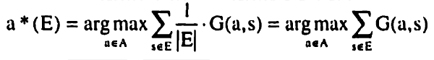
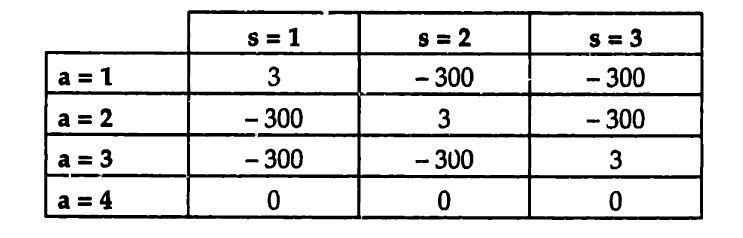
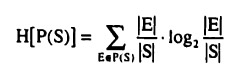
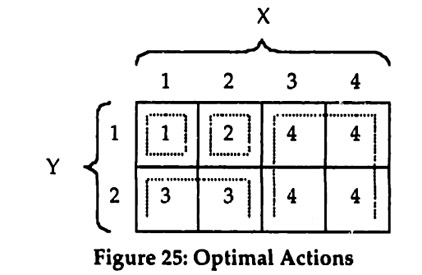
SY, where Sx = {1, 2,3,4} and SY = {1,2}. This two dimensional state space represents the information observed by the two team members X and Y. Let the set of actions be given by A = {1,2,3,4}. Finally, to keep the example really simple, assume that the benefit function is represented by the matrix in Figure 25, where the action shown for each cell has a benefit of 1 in that cell and all other actions have no benefit. It follows immediately that Figure 25 shows the optimal action for each possible state.

Also shown in Figure 25 are constant action subsets for each of the optimal actions, as indicated by the dotted lines. Since a communication protocol will again consist of bisections, it follows by induction that only "rectangles" are well-formed constant action subsets, where a rectangle is given by Ex \otimes \!\, EY where Ex is a subset of Sx and EY of SY respectively. 37

Cost minimizing protocols can again be determined by an approach similar to that introduced in Section 5 above. In this simple example, it will further be assumed that the cost of communication is sufficiently low that a partition into the indicated constant action subsets is possible. The focus will be on the cost-minimizing protocol. Building the protocol "bottom-up" by starting with the constant action subsets and combining subsequently larger sub-trees results in the protocol show in Figure 26.

37 Note that a rectangle does not have to be a geographic rectangle in diagrams like Figure 25, since columns and rows do not need to be adjacent.

The optimal protocol constructed this way has the feature that the communication alternates between the two team members X and Y. This can be interpreted as synchronous communication, which requires both parties to simultaneously participate in the communication. Given the assumed uniform distribution, it can be seen by inspection that the expected message length is (8/8) • 1 + (4/8) • 2 + (2/8) • 3 = 22/8 = 2.75.

Figure 27 shows an alternative asynchronous protocol, where team member Y starts by sending the available information and team member X responds at some later point.

Again, the expected total message length for the asynchronous protocol from Figure 27, can be determined by inspection as (2/2) • 1 + (4/4) • 1 + (2/4) • 2 = 3. The asynchronous protocol thus has a higher cost of communication than the optimal protocol determined using the "bottom-up" construction approach.

The example obviously only scratches the surface of bi-directional communication. Nevertheless, it serves to illustrate the additional complexity that results from having distributed information. While the key difficulty lies again in simultaneously determining the benefit and the cost of different protocols and optimizing over the space of all protocols, this turns out to be significantly more difficult in the two dimensional case.

7.3 Outlook

An ideal goal for further research is to use the protocol-based approach to derive simplified models of communication cost that are nevertheless grounded in fundamentals. Much like Holmstrom and Milgrom's paper on "Aggregation and Linearity" (1987) paved the way for studying a large number of incentive problems using simple linear schemes, such a result would greatly contribute to the exploration of communication problems.

APPENDIX

A1. Cost of Coding

Claim: For any partition P(S), the cost of coding is independent of the structure of the protocol and is given by

E [Cc(m(x,Ψ), Ψ)] = cc • H [P(S)]

where H[ • ] is the entropy of the partition P(S).

Proof: By induction on | P(S) |. Assume without loss of generality that cc = 1 to simplify notation. Base case: | P(S) | = 1. If P(S) has only one element, it must be S, so H[P(S)] = 1 • log 1 = 0. This is the correct cost, since no coding is required and hence the claim is true for the base case. Inductive hypothesis: |P(S) | = n. Assume the claim is true when P(S) has n elements. Induction: | P(S) | = n + 1. Consider the binary tree Ψ for a protocol that implements P(S) and assume without loss of generality that Ψ is a full binary tree, i.e. each non-terminal node has two children (any nodes with only one child can be eliminated). Find a non-terminal node N so that both children of N are terminal nodes. A full binary tree is guaranteed to have at least one such node. Denote the elements of the partition P(S) at the two terminal nodes as E1 and E2. Let E = E1 U E2. Let p = |E1 | / |E|. Then the cost of coding incurred at N is h(p). Now, consider the tree Ψ' where N is replaced by a terminal node with the subset E, so that implements P'(S) which has n elements. Using the inductive hypothesis, it follows that E[CC(Ψ', s)] = H[P'(S)]. The expected cost of coding for y can now be derived as follows:

A2. Counterexample for Greedy Algorithm

Consider the following matrix of benefits for various combinations of states and actions.

  s = l s = 2 s = 3 s = 4
a = l 3 -1000 -1000 -1000
a = 2 1 1 -1000 -1000
a = 3 -1000 -1000 2 -1000
a = 4 -1000 -1000 -1000 2
a = 5 0 0 0 0

Assume further that the cost of communication are non-zero but sufficiently low to allow for at least two bisections.

The following table lists the benefits from all possible first bisections (these can easily be derived by inspection).

E1 E2 Benefit
{1} {2,3,4} 3/4
{2} {1,3,4} 1/4
{3} {1,2,4} 2/4 = 1/2
{4} {1,2,3} 2/4 = 1/2
{1,2} {3,4} 1/4 + 1/4 = 1/2
{1,3} {2,4} 0/4 = 0
{1,4} {2,3} 0/4 = 0

The optimal first bisection is clearly E1 = {1} and E2 = {2,3,4}, since it has the highest marginal benefit and the lowest marginal cost.
Now consider the marginal benefits from a second bisection, given that the optimal first bisection was chosen.

E1' E2' Benefit
{2} {3,4} 1/4
{3} {2,4} 2/4 = 1/2
{4} {2,3} 2/4 = 1/2

Hence the maximal total benefit after having chosen the optimal first bisection is 3/4 + 1/2 = 5/4. Contrast this with the total benefit from the partition {{1, 2}, {3}, {4}}, which can easily be verified to be 6/4. Since this partition can only be achieved by choosing a sub-optimal first bisection, it follows immediately that a greedy algorithm based on the optimal bisection as defined here cannot be successful.

A3. Historical Cost of Communication

Based on the Historical Statistics of the United States (1976), the rates for letters in 1908 were 2 cents per 1/2 oz., independent of distance within the 50 states. A 1/2 oz. letter can contain three to four pages of paper, which with average handwriting or single-spaced typing can hold upward of 1,500 words. The cost of transmission is thus essentially fixed and extremely low. Telegrams on the other hand were restricted to ten words or fewer. In 1908 the rate for a telegram from New York City to Chicago was 50 cents and to San Francisco it was 100 cents. The restriction to ten or fewer words means that the cost of transmission is effectively variable with an average rate of 5 to 10 cents per word. In 1908 the telephone was a possible alternative to letters and telegrams, but it was not yet in widespread use. Its adoption had been slowed down by high rates for the installation and rental of handsets, as well as the high long distance usage rates.

REFERENCES

Brynjolfsson, E. and L. Hitt (1996). "IT and Organizational Architecture." mimeo.
Chandler, A. D. J. (1977). The Visible Hand. Cambridge, Massachusetts, Harvard University Press.
Cormen, T. H., C. E. Leierson, et al. (1990). Introduction to Algorithms. Cambridge, The MIT Press.
Green, J. and J.-J. Laffont (1986). Incentive theory with data compression.
Uncertainty, information, and communication. W. P. Heller, R. M. Starr and D. A. Starrett Cambridge, Cambridge University press: 239-253.
Green, J. and J.-J. Laffont (1987). Limited Communication and Incentive
Compatibility. Information, Incentives, and Economic Mechanisms. T. Groves, R. Radner and S. Reiter, Minneapolis, University of Minnesota Press: 308-329.
Historical Statistics of the United States (1976). Bicentennial edition, published by the U.S. Department of Commerce, Bureau of the Census. Washington, D.C.
Holmstrom, B. and P. Milgrom (1987). "Aggregation and Linearity in the Provision of Intertemporal Incentives." Econometrica 55(2): 303-28.
Huffman, D, A. (1952). "A Method for the Construction of Minimum-Redundancy Codes." Proceedings IRE 40(9 (Sept.)): 1098-1101.
Hurwicz, L. (1986). On informational decentralization and effiency in resource allocation mechanisms. Studies in Mathematical Economics. S, Reiter. Providence, The Mathematical Association of America.
Kreps, D. M. (1990). A Course in Microeconomic Theory. Princeton, Princeton University Press.
Malone, T. and S. Smith (1988). "Modeling the Performance of Organizational Structures." Operations Research 36(3): 421-436.
Malone, T. and G. Wyner (1996). "Control, Empowerment, and Information Technology." mimeo.
Marschak, J. and R. Radner (1972). Economic Theory of Teams. New Haven, Yale University Press.
McLuhan, M. (1962). The Gutenberg Galaxy: The Making of Typographic Man. Toronto, University of Toronto Press.
Segal, I. (1996). "Communication Complexity and Coordination by Authority."
Department of Economics, University of California at Berkeley mimeo.
Shannon, C. (1948). "A Mathematical Theory of Communication." Bell Systems Technical Tournal(27): 379-423.
Van Zandt, T. (1997). Decentralized Information Processing in the Theory of Organizations. Contemporary Economic Development Reviewed. M.
Sertel. London, MacMillan Press. Vol 4: The Enterprise and its Environment.
Yao, A. C. (1979). "Some Complexity Questions Related to Distributive
Computing." Proceedings of the Uth ACM Symposium on the Theory of Computing: 209-213.
Yates (1989), Control through Communication: The Rise of System in American Management. Baltimore, Johns Hopkins University Press.
Yates, J. and W. J. Orlikowski (1992). "Genres of Organizational Communication: A Structurational Approach to Sutdying Communication and Media." Academy of Management Review 17(2): 299-326.